Statistical learning theory
| Machine learning and data mining |
|---|
 |
|
Machine-learning venues |
Statistical learning theory is a framework for machine learning drawing from the fields of statistics and functional analysis.[1][2] Statistical learning theory deals with the problem of finding a predictive function based on data. Statistical learning theory has led to successful applications in fields such as computer vision, speech recognition, bioinformatics and baseball.[3]
Contents
Introduction[edit]
The goals of learning are understanding and prediction. Learning falls into many categories, including supervised learning, unsupervised learning, online learning, and reinforcement learning. From the perspective of statistical learning theory, supervised learning is best understood.[4] Supervised learning involves learning from a training set of data. Every point in the training is an input-output pair, where the input maps to an output. The learning problem consists of inferring the function that maps between the input and the output, such that the learned function can be used to predict the output from future input.
Depending on the type of output, supervised learning problems are either problem of regression or problems of classification. If the output takes a continuous range of values, it is a regression problem. Using Ohm's Law as an example, a regression could be performed with voltage as input and current as an output. The regression would find the functional relationship between voltage and current to be , such that
Classification problems are those for which the output will be an element from a discrete set of labels. Classification is very common for machine learning applications. In facial recognition, for instance, a picture of a person's face would be the input, and the output label would be that person's name. The input would be represented by a large multidimensional vector whose elements represent pixels in the picture.
After learning a function based on the training set data, that function is validated on a test set of data, data that did not appear in the training set.
Formal description[edit]
Take to be the vector space of all possible inputs, and to be the vector space of all possible outputs. Statistical learning theory takes the perspective that there is some unknown probability distribution over the product space , i.e. there exists some unknown . The training set is made up of samples from this probability distribution, and is notated
Every is an input vector from the training data, and is the output that corresponds to it.
In this formalism, the inference problem consists of finding a function such that . Let be a space of functions called the hypothesis space. The hypothesis space is the space of functions the algorithm will search through. Let be the loss function, a metric for the difference between the predicted value and the actual value . The expected risk is defined to be
The target function, the best possible function that can be chosen, is given by the that satisfies
Because the probability distribution is unknown, a proxy measure for the expected risk must be used. This measure is based on the training set, a sample from this unknown probability distribution. It is called the empirical risk
A learning algorithm that chooses the function that minimizes the empirical risk is called empirical risk minimization.
Loss functions[edit]
The choice of loss function is a determining factor on the function that will be chosen by the learning algorithm. The loss function also affects the convergence rate for an algorithm. It is important for the loss function to be convex.[5]
Different loss functions are used depending on whether the problem is one of regression or one of classification.
Regression[edit]
The most common loss function for regression is the square loss function (also known as the L2-norm). This familiar loss function is used in ordinary least squares regression. The form is:
The absolute value loss (also known as the L1-norm) is also sometimes used:
Classification[edit]
In some sense the 0-1 indicator function is the most natural loss function for classification. It takes the value 0 if the predicted output is the same as the actual output, and it takes the value 1 if the predicted output is different from the actual output. For binary classification with , this is:
where is the Heaviside step function.
Regularization[edit]
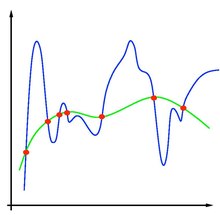
In machine learning problems, a major problem that arises is that of overfitting. Because learning is a prediction problem, the goal is not to find a function that most closely fits the (previously observed) data, but to find one that will most accurately predict output from future input. Empirical risk minimization runs this risk of overfitting: finding a function that matches the data exactly but does not predict future output well.
Overfitting is symptomatic of unstable solutions; a small perturbation in the training set data would cause a large variation in the learned function. It can be shown that if the stability for the solution can be guaranteed, generalization and consistency are guaranteed as well.[6][7] Regularization can solve the overfitting problem and give the problem stability.
Regularization can be accomplished by restricting the hypothesis space . A common example would be restricting to linear functions: this can be seen as a reduction to the standard problem of linear regression. could also be restricted to polynomial of degree , exponentials, or bounded functions on L1. Restriction of the hypothesis space avoids overfitting because the form of the potential functions are limited, and so does not allow for the choice of a function that gives empirical risk arbitrarily close to zero.
One example of regularization is Tikhonov regularization. This consists of minimizing
where is a fixed and positive parameter, the regularization parameter. Tikhonov regularization ensures existence, uniqueness, and stability of the solution.[8]
See also[edit]
- Reproducing kernel Hilbert spaces are a useful choice for .
- Proximal gradient methods for learning
References[edit]
- ^ Trevor Hastie, Robert Tibshirani, Jerome Friedman (2009) The Elements of Statistical Learning, Springer-Verlag ISBN 978-0-387-84857-0.
- ^ Mohri, Mehryar; Rostamizadeh, Afshin; Talwalkar, Ameet (2012). Foundations of Machine Learning. USA, Massachusetts: MIT Press. ISBN 9780262018258.
- ^ Gagan Sidhu, Brian Caffo. Exploiting pitcher decision-making using Reinforcement Learning. Annals of Applied Statistics
- ^ Tomaso Poggio, Lorenzo Rosasco, et al. Statistical Learning Theory and Applications, 2012, Class 1
- ^ Rosasco, L., Vito, E.D., Caponnetto, A., Fiana, M., and Verri A. 2004. Neural computation Vol 16, pp 1063-1076
- ^ Vapnik, V.N. and Chervonenkis, A.Y. 1971. On the uniform convergence of relative frequencies of events to their probabilities. Theory of Probability and its Applications Vol 16, pp 264-280.
- ^ Mukherjee, S., Niyogi, P. Poggio, T., and Rifkin, R. 2006. Learning theory: stability is sufficient for generalization and necessary and sufficient for consistency of empirical risk minimization. Advances in Computational Mathematics. Vol 25, pp 161-193.
- ^ Tomaso Poggio, Lorenzo Rosasco, et al. Statistical Learning Theory and Applications, 2012, Class 2


![{\displaystyle I[f]=\displaystyle \int _{X\times Y}V(f({\vec {x}}),y)\,p({\vec {x}},y)\,d{\vec {x}}\,dy}](https://wikimedia.org/api/rest_v1/media/math/render/svg/7c97de659352fa60d6624a1f54f4d3f0b32c73af)

![{\displaystyle f=\inf _{h\in {\mathcal {H}}}I[h]}](https://wikimedia.org/api/rest_v1/media/math/render/svg/47c982d6049c9ce70930b327589b5ff00915406f)

![I_{S}[f]={\frac {1}{n}}\displaystyle \sum _{{i=1}}^{n}V(f({\vec {x}}_{i}),y_{i})](https://wikimedia.org/api/rest_v1/media/math/render/svg/0418e949bbea67e3cdbe4455429c3af2c3f09781)


