File:Lagrange very simple.svg

Summary

DescriptionLagrange very simple.svg	Català: Fig. 2. Il·lustració del problema d'optimització restringida. English: Fig. 3. Illustration of the constrained optimization problem. Italiano: Figura 3. Illustrazione del problema di ottimizzazione vincolata. Nederlands: Afbeelding 3: eenvoudig voorbeeld. Polski: Wykresem funkcji jest płaszczyzna. W przestrzeni trójwymiarowej, równanie opisuje walec (u którego podstawy, na płaszczyźnie leży okrąg jednostkowy). Szukanie ekstremów warunkowych sprowadza się w tym wypadku do badania punktów ekstremalnych części wspólnej walca i płaszczyzny.
Date	7 August 2012, 17:11 (UTC)
Source	This file was derived from: Lagrange very simple.jpg:
Author	Lagrange_very_simple.jpg: User:Jacobmelgaard derivative work: Zerodamage

This is a retouched picture, which means that it has been digitally altered from its original version. Modifications: Vectorization. The original can be viewed here: Lagrange very simple.jpg. Modifications made by Zerodamage.

Licensing

I, the copyright holder of this work, hereby publish it under the following licenses:

	This file is licensed under the Creative Commons Attribution-Share Alike 3.0 Unported license.
	You are free: to share – to copy, distribute and transmit the work to remix – to adapt the work Under the following conditions: attribution – You must give appropriate credit, provide a link to the license, and indicate if changes were made. You may do so in any reasonable manner, but not in any way that suggests the licensor endorses you or your use. share alike – If you alter, transform, or build upon this work, you may distribute the resulting work only under the same or similar license to this one.
	This licensing tag was added to this file as part of the GFDL licensing update.http://creativecommons.org/licenses/by-sa/3.0/CC-BY-SA-3.0Creative Commons Attribution-Share Alike 3.0truetrue

Permission is granted to copy, distribute and/or modify this document under the terms of the GNU Free Documentation License, Version 1.2 or any later version published by the Free Software Foundation; with no Invariant Sections, no Front-Cover Texts, and no Back-Cover Texts. A copy of the license is included in the section entitled GNU Free Documentation License.http://www.gnu.org/copyleft/fdl.htmlGFDLGNU Free Documentation Licensetruetrue

You may select the license of your choice.

Source code

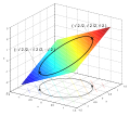
The graph was made in Matlab with the following source code. Corrected in Inkscape

% Function data
[X,Y] = meshgrid(-1.2:0.1:1.2, -1.2:0.1:1.2);
Z = X+Y;

% Constraint data
t = -pi:0.01:pi;
xc = cos(t);
yc = sin(t);
zc = xc+yc;

% Plot graph and 'constraint'
figure();
surfc(X,Y,Z);
hold on;
plot3(xc, yc, zc, 'k', 'LineWidth', 2);
plot3(xc, yc, -3*ones(1,length(t)), 'k', 'LineWidth', 1);
set(1, 'Color', [1 1 1]);
set(1, 'Position', [46 107 767 682]);
% Axis labels
text(0.2, -2.2, -3, 'x');
text(2.0, -.3, -3, 'y');
text(-1.8, -1.5, 0, 'z');

% Annotations of the max and min points
% Point indicating max
plot3(sqrt(2)/2, sqrt(2)/2, 1.45, 'kx', 'MarkerSize', 14, 'LineWidth', 2);
plot3(sqrt(2)/2, sqrt(2)/2, -3, 'kx', 'MarkerSize', 10, 'LineWidth', 2);
text('Interpreter', 'latex', 'String', '$$(\sqrt{2}/2, \sqrt{2}/2, \sqrt{2})$$',...
        'Position', [.0 .3 1.9], 'FontSize', 20);
% Point indicating min
plot3(-sqrt(2)/2, -sqrt(2)/2, -sqrt(2), 'kx', 'MarkerSize', 14, 'LineWidth', 2);
plot3(-sqrt(2)/2, -sqrt(2)/2, -3, 'kx', 'MarkerSize', 10, 'LineWidth', 2);
text('Interpreter', 'latex', 'String', '$$(-\sqrt{2}/2, -\sqrt{2}/2, -\sqrt{2})$$',...
        'Position', [-1.4 -1.0 -1.0], 'FontSize', 20);
hold off

view([34 24]);

%interpolate for improved rendering
shading interp;

%plot2svg must be retrieved from http://www.zhinst.com/blogs/schwizer/
plot2svg;

Original upload log

This image is a derivative work of the following images:

• File:Lagrange_very_simple.jpg licensed with Cc-by-sa-3.0-migrated, GFDL
  • 2007-09-20T13:31:36Z Loxley 685x597 (67879 Bytes) {{Information |Description= |Source=The graph was made in Matlab with the following source code % Function data [X,Y] = meshgrid(-1.2:0.01:1.2, -1.2:0.01:1.2); Z = XY; % Constraint data t = -pi:0.01:pi; xc = cos(t); yc = s

Uploaded with derivativeFX