Artificial neural network
| Machine learning and data mining |
|---|
 |
|
Machine-learning venues |

Artificial neural networks (ANN) or connectionist systems are computing systems vaguely inspired by the biological neural networks that constitute animal brains.[1] The neural network itself is not an algorithm, but rather a framework for many different machine learning algorithms to work together and process complex data inputs.[2] Such systems "learn" to perform tasks by considering examples, generally without being programmed with any task-specific rules. For example, in image recognition, they might learn to identify images that contain cats by analyzing example images that have been manually labeled as "cat" or "no cat" and using the results to identify cats in other images. They do this without any prior knowledge about cats, for example, that they have fur, tails, whiskers and cat-like faces. Instead, they automatically generate identifying characteristics from the learning material that they process.
An ANN is based on a collection of connected units or nodes called artificial neurons, which loosely model the neurons in a biological brain. Each connection, like the synapses in a biological brain, can transmit a signal from one artificial neuron to another. An artificial neuron that receives a signal can process it and then signal additional artificial neurons connected to it.
In common ANN implementations, the signal at a connection between artificial neurons is a real number, and the output of each artificial neuron is computed by some non-linear function of the sum of its inputs. The connections between artificial neurons are called 'edges'. Artificial neurons and edges typically have a weight that adjusts as learning proceeds. The weight increases or decreases the strength of the signal at a connection. Artificial neurons may have a threshold such that the signal is only sent if the aggregate signal crosses that threshold. Typically, artificial neurons are aggregated into layers. Different layers may perform different kinds of transformations on their inputs. Signals travel from the first layer (the input layer), to the last layer (the output layer), possibly after traversing the layers multiple times.
The original goal of the ANN approach was to solve problems in the same way that a human brain would. However, over time, attention moved to performing specific tasks, leading to deviations from biology. Artificial neural networks have been used on a variety of tasks, including computer vision, speech recognition, machine translation, social network filtering, playing board and video games and medical diagnosis.
Contents
- 1 History
- 2 Models
- 3 Optimization
- 4 Algorithm in code
- 5 Extension
- 6 Modes of learning
- 7 Variants
- 7.1 Group method of data handling
- 7.2 Convolutional neural networks
- 7.3 Long short-term memory
- 7.4 Deep reservoir computing
- 7.5 Deep belief networks
- 7.6 Large memory storage and retrieval neural networks
- 7.7 Stacked (de-noising) auto-encoders
- 7.8 Deep stacking networks
- 7.9 Tensor deep stacking networks
- 7.10 Spike-and-slab RBMs
- 7.11 Compound hierarchical-deep models
- 7.12 Deep predictive coding networks
- 7.13 Networks with separate memory structures
- 7.14 Multilayer kernel machine
- 8 Neural architecture search
- 9 Use
- 10 Applications
- 11 Theoretical properties
- 12 Criticism
- 13 Types
- 14 Gallery
- 15 See also
- 16 References
- 17 Bibliography
History[edit]
Warren McCulloch and Walter Pitts[3] (1943) created a computational model for neural networks based on mathematics and algorithms called threshold logic. This model paved the way for neural network research to split into two approaches. One approach focused on biological processes in the brain while the other focused on the application of neural networks to artificial intelligence. This work led to work on nerve networks and their link to finite automata.[4]
Hebbian learning[edit]
In the late 1940s, D. O. Hebb[5] created a learning hypothesis based on the mechanism of neural plasticity that became known as Hebbian learning. Hebbian learning is unsupervised learning. This evolved into models for long term potentiation. Researchers started applying these ideas to computational models in 1948 with Turing's B-type machines. Farley and Clark[6] (1954) first used computational machines, then called "calculators", to simulate a Hebbian network. Other neural network computational machines were created by Rochester, Holland, Habit and Duda (1956).[7] Rosenblatt[8] (1958) created the perceptron, an algorithm for pattern recognition. With mathematical notation, Rosenblatt described circuitry not in the basic perceptron, such as the exclusive-or circuit that could not be processed by neural networks at the time.[9] In 1959, a biological model proposed by Nobel laureates Hubel and Wiesel was based on their discovery of two types of cells in the primary visual cortex: simple cells and complex cells.[10] The first functional networks with many layers were published by Ivakhnenko and Lapa in 1965, becoming the Group Method of Data Handling.[11][12][13]
Neural network research stagnated after machine learning research by Minsky and Papert (1969),[14] who discovered two key issues with the computational machines that processed neural networks. The first was that basic perceptrons were incapable of processing the exclusive-or circuit. The second was that computers didn't have enough processing power to effectively handle the work required by large neural networks. Neural network research slowed until computers achieved far greater processing power. Much of artificial intelligence had focused on high-level (symbolic) models that are processed by using algorithms, characterized for example by expert systems with knowledge embodied in if-then rules, until in the late 1980s research expanded to low-level (sub-symbolic) machine learning, characterized by knowledge embodied in the parameters of a cognitive model.[citation needed]
Backpropagation[edit]
A key trigger for renewed interest in neural networks and learning was Werbos's (1975) backpropagation algorithm that effectively solved the exclusive-or problem by making the training of multi-layer networks feasible and efficient. Backpropagation distributed the error term back up through the layers, by modifying the weights at each node.[9]
In the mid-1980s, parallel distributed processing became popular under the name connectionism. Rumelhart and McClelland (1986) described the use of connectionism to simulate neural processes.[15]
Support vector machines and other, much simpler methods such as linear classifiers gradually overtook neural networks in machine learning popularity. However, using neural networks transformed some domains, such as the prediction of protein structures.[16][17]
In 1992, max-pooling was introduced to help with least shift invariance and tolerance to deformation to aid in 3D object recognition.[18][19][20] In 2010, Backpropagation training through max-pooling was accelerated by GPUs and shown to perform better than other pooling variants.[21]
The vanishing gradient problem affects many-layered feedforward networks that used backpropagation and also recurrent neural networks (RNNs).[22][23] As errors propagate from layer to layer, they shrink exponentially with the number of layers, impeding the tuning of neuron weights that is based on those errors, particularly affecting deep networks.
To overcome this problem, Schmidhuber adopted a multi-level hierarchy of networks (1992) pre-trained one level at a time by unsupervised learning and fine-tuned by backpropagation.[24] Behnke (2003) relied only on the sign of the gradient (Rprop)[25] on problems such as image reconstruction and face localization.
Hinton et al. (2006) proposed learning a high-level representation using successive layers of binary or real-valued latent variables with a restricted Boltzmann machine[26] to model each layer. Once sufficiently many layers have been learned, the deep architecture may be used as a generative model by reproducing the data when sampling down the model (an "ancestral pass") from the top level feature activations.[27][28] In 2012, Ng and Dean created a network that learned to recognize higher-level concepts, such as cats, only from watching unlabeled images taken from YouTube videos.[29]
Earlier challenges in training deep neural networks were successfully addressed with methods such as unsupervised pre-training, while available computing power increased through the use of GPUs and distributed computing. Neural networks were deployed on a large scale, particularly in image and visual recognition problems. This became known as "deep learning".[citation needed]
Hardware-based designs[edit]
Computational devices were created in CMOS, for both biophysical simulation and neuromorphic computing. Nanodevices[30] for very large scale principal components analyses and convolution may create a new class of neural computing because they are fundamentally analog rather than digital (even though the first implementations may use digital devices).[31] Ciresan and colleagues (2010)[32] in Schmidhuber's group showed that despite the vanishing gradient problem, GPUs makes back-propagation feasible for many-layered feedforward neural networks.
Contests[edit]
Between 2009 and 2012, recurrent neural networks and deep feedforward neural networks developed in Schmidhuber's research group won eight international competitions in pattern recognition and machine learning.[33][34] For example, the bi-directional and multi-dimensional long short-term memory (LSTM)[35][36][37][38] of Graves et al. won three competitions in connected handwriting recognition at the 2009 International Conference on Document Analysis and Recognition (ICDAR), without any prior knowledge about the three languages to be learned.[37][36]
Ciresan and colleagues won pattern recognition contests, including the IJCNN 2011 Traffic Sign Recognition Competition,[39] the ISBI 2012 Segmentation of Neuronal Structures in Electron Microscopy Stacks challenge[40] and others. Their neural networks were the first pattern recognizers to achieve human-competitive or even superhuman performance[41] on benchmarks such as traffic sign recognition (IJCNN 2012), or the MNIST handwritten digits problem.
Researchers demonstrated (2010) that deep neural networks interfaced to a hidden Markov model with context-dependent states that define the neural network output layer can drastically reduce errors in large-vocabulary speech recognition tasks such as voice search.
GPU-based implementations[42] of this approach won many pattern recognition contests, including the IJCNN 2011 Traffic Sign Recognition Competition,[39] the ISBI 2012 Segmentation of neuronal structures in EM stacks challenge,[40] the ImageNet Competition[43] and others.
Deep, highly nonlinear neural architectures similar to the neocognitron[44] and the "standard architecture of vision",[45] inspired by simple and complex cells, were pre-trained by unsupervised methods by Hinton.[46][27] A team from his lab won a 2012 contest sponsored by Merck to design software to help find molecules that might identify new drugs.[47]
Convolutional networks[edit]
As of 2011[update], the state of the art in deep learning feedforward networks alternated between convolutional layers and max-pooling layers,[42][48] topped by several fully or sparsely connected layers followed by a final classification layer. Learning is usually done without unsupervised pre-training. In the convolutional layer, there are filters that are convolved with the input. Each filter is equivalent to a weights vector that has to be trained.
Such supervised deep learning methods were the first to achieve human-competitive performance on certain tasks.[41]
Artificial neural networks were able to guarantee shift invariance to deal with small and large natural objects in large cluttered scenes, only when invariance extended beyond shift, to all ANN-learned concepts, such as location, type (object class label), scale, lighting and others. This was realized in Developmental Networks (DNs)[49] whose embodiments are Where-What Networks, WWN-1 (2008)[50] through WWN-7 (2013).[51]
Models[edit]
This section may be confusing or unclear to readers. (April 2017) (Learn how and when to remove this template message) |

An artificial neural network is a network of simple elements called artificial neurons, which receive input, change their internal state (activation) according to that input, and produce output depending on the input and activation.
An artificial neuron mimics the working of a biophysical neuron with inputs and outputs, but is not a biological neuron model.
The network forms by connecting the output of certain neurons to the input of other neurons forming a directed, weighted graph. The weights as well as the functions that compute the activation can be modified by a process called learning which is governed by a learning rule.[52]
Components of an artificial neural network[edit]
Neurons[edit]
A neuron with label receiving an input from predecessor neurons consists of the following components:[52]


- an activation , the neuron's state, depending on a discrete time parameter,
- possibly a threshold , which stays fixed unless changed by a learning function,
- an activation function that computes the new activation at a given time from , and the net input giving rise to the relation


- ,

- and an output function computing the output from the activation

- .

Often the output function is simply the Identity function.
An input neuron has no predecessor but serves as input interface for the whole network. Similarly an output neuron has no successor and thus serves as output interface of the whole network.
Connections, weights and biases[edit]
The network consists of connections, each connection transferring the output of a neuron to the input of a neuron . In this sense is the predecessor of and is the successor of . Each connection is assigned a weight .[52] Sometimes a bias term is added to the total weighted sum of inputs to serve as a threshold to shift the activation function.[53]


Propagation function[edit]
The propagation function computes the input to the neuron from the outputs of predecessor neurons and typically has the form[52]

- .

When a bias value is added with the function, the above form changes to the following [54]
- , where is a bias.


Learning rule[edit]
The learning rule is a rule or an algorithm which modifies the parameters of the neural network, in order for a given input to the network to produce a favored output. This learning process typically amounts to modifying the weights and thresholds of the variables within the network.[52]
Neural networks as functions[edit]
Neural network models can be viewed as simple mathematical models defining a function or a distribution over or both and . Sometimes models are intimately associated with a particular learning rule. A common use of the phrase "ANN model" is really the definition of a class of such functions (where members of the class are obtained by varying parameters, connection weights, or specifics of the architecture such as the number of neurons or their connectivity).


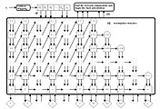
Mathematically, a neuron's network function is defined as a composition of other functions , that can further be decomposed into other functions. This can be conveniently represented as a network structure, with arrows depicting the dependencies between functions. A widely used type of composition is the nonlinear weighted sum, where , where (commonly referred to as the activation function[55]) is some predefined function, such as the hyperbolic tangent or sigmoid function or softmax function or rectifier function. The important characteristic of the activation function is that it provides a smooth transition as input values change, i.e. a small change in input produces a small change in output. The following refers to a collection of functions as a vector .


.svg)
This figure depicts such a decomposition of , with dependencies between variables indicated by arrows. These can be interpreted in two ways.

The first view is the functional view: the input is transformed into a 3-dimensional vector , which is then transformed into a 2-dimensional vector , which is finally transformed into . This view is most commonly encountered in the context of optimization.


The second view is the probabilistic view: the random variable depends upon the random variable , which depends upon , which depends upon the random variable . This view is most commonly encountered in the context of graphical models.


The two views are largely equivalent. In either case, for this particular architecture, the components of individual layers are independent of each other (e.g., the components of are independent of each other given their input ). This naturally enables a degree of parallelism in the implementation.

Networks such as the previous one are commonly called feedforward, because their graph is a directed acyclic graph. Networks with cycles are commonly called recurrent. Such networks are commonly depicted in the manner shown at the top of the figure, where is shown as being dependent upon itself. However, an implied temporal dependence is not shown.
Learning[edit]
The possibility of learning has attracted the most interest in neural networks. Given a specific task to solve, and a class of functions , learning means using a set of observations to find which solves the task in some optimal sense.


This entails defining a cost function such that, for the optimal solution , – i.e., no solution has a cost less than the cost of the optimal solution (see mathematical optimization).


The cost function is an important concept in learning, as it is a measure of how far away a particular solution is from an optimal solution to the problem to be solved. Learning algorithms search through the solution space to find a function that has the smallest possible cost.

For applications where the solution is data dependent, the cost must necessarily be a function of the observations, otherwise the model would not relate to the data. It is frequently defined as a statistic to which only approximations can be made. As a simple example, consider the problem of finding the model , which minimizes , for data pairs drawn from some distribution . In practical situations we would only have samples from and thus, for the above example, we would only minimize . Thus, the cost is minimized over a sample of the data rather than the entire distribution.
![\textstyle C=E\left[(f(x)-y)^{2}\right]](https://wikimedia.org/api/rest_v1/media/math/render/svg/53d492067dfb4b20e428a37d76787463e95c8d18)


When some form of online machine learning must be used, where the cost is reduced as each new example is seen. While online machine learning is often used when is fixed, it is most useful in the case where the distribution changes slowly over time. In neural network methods, some form of online machine learning is frequently used for finite datasets.

Choosing a cost function[edit]
While it is possible to define an ad hoc cost function, frequently a particular cost function is used, either because it has desirable properties (such as convexity) or because it arises naturally from a particular formulation of the problem (e.g., in a probabilistic formulation the posterior probability of the model can be used as an inverse cost). Ultimately, the cost function depends on the task.
Backpropagation[edit]
A DNN can be discriminatively trained with the standard backpropagation algorithm. Backpropagation is a method to calculate the gradient of the loss function (produces the cost associated with a given state) with respect to the weights in an ANN.
The basics of continuous backpropagation[11][56][57][58] were derived in the context of control theory by Kelley[59] in 1960 and by Bryson in 1961,[60] using principles of dynamic programming. In 1962, Dreyfus published a simpler derivation based only on the chain rule.[61] Bryson and Ho described it as a multi-stage dynamic system optimization method in 1969.[62][63] In 1970, Linnainmaa finally published the general method for automatic differentiation (AD) of discrete connected networks of nested differentiable functions.[64][65] This corresponds to the modern version of backpropagation which is efficient even when the networks are sparse.[11][56][66][67] In 1973, Dreyfus used backpropagation to adapt parameters of controllers in proportion to error gradients.[68] In 1974, Werbos mentioned the possibility of applying this principle to Artificial neural networks,[69] and in 1982, he applied Linnainmaa's AD method to neural networks in the way that is widely used today.[56][70] In 1986, Rumelhart, Hinton and Williams noted that this method can generate useful internal representations of incoming data in hidden layers of neural networks.[71] In 1993, Wan was the first[11] to win an international pattern recognition contest through backpropagation.[72]
The weight updates of backpropagation can be done via stochastic gradient descent using the following equation:

where, is the learning rate, is the cost (loss) function and a stochastic term. The choice of the cost function depends on factors such as the learning type (supervised, unsupervised, reinforcement, etc.) and the activation function. For example, when performing supervised learning on a multiclass classification problem, common choices for the activation function and cost function are the softmax function and cross entropy function, respectively. The softmax function is defined as where represents the class probability (output of the unit ) and and represent the total input to units and of the same level respectively. Cross entropy is defined as where represents the target probability for output unit and is the probability output for after applying the activation function.[73]


These can be used to output object bounding boxes in the form of a binary mask. They are also used for multi-scale regression to increase localization precision. DNN-based regression can learn features that capture geometric information in addition to serving as a good classifier. They remove the requirement to explicitly model parts and their relations. This helps to broaden the variety of objects that can be learned. The model consists of multiple layers, each of which has a rectified linear unit as its activation function for non-linear transformation. Some layers are convolutional, while others are fully connected. Every convolutional layer has an additional max pooling. The network is trained to minimize L2 error for predicting the mask ranging over the entire training set containing bounding boxes represented as masks.
Alternatives to backpropagation include Extreme Learning Machines,[74] "No-prop" networks,[75] training without backtracking,[76] "weightless" networks,[77][78] and non-connectionist neural networks.
Learning paradigms[edit]
The three major learning paradigms each correspond to a particular learning task. These are supervised learning, unsupervised learning and reinforcement learning.
Supervised learning[edit]
Supervised learning uses a set of example pairs and the aim is to find a function in the allowed class of functions that matches the examples. In other words, we wish to infer the mapping implied by the data; the cost function is related to the mismatch between our mapping and the data and it implicitly contains prior knowledge about the problem domain.[79]


A commonly used cost is the mean-squared error, which tries to minimize the average squared error between the network's output, , and the target value over all the example pairs. Minimizing this cost using gradient descent for the class of neural networks called multilayer perceptrons (MLP), produces the backpropagation algorithm for training neural networks.


Tasks that fall within the paradigm of supervised learning are pattern recognition (also known as classification) and regression (also known as function approximation). The supervised learning paradigm is also applicable to sequential data (e.g., for hand writing, speech and gesture recognition). This can be thought of as learning with a "teacher", in the form of a function that provides continuous feedback on the quality of solutions obtained thus far.
Unsupervised learning[edit]
In unsupervised learning, some data is given and the cost function to be minimized, that can be any function of the data and the network's output, .
The cost function is dependent on the task (the model domain) and any a priori assumptions (the implicit properties of the model, its parameters and the observed variables).
As a trivial example, consider the model where is a constant and the cost . Minimizing this cost produces a value of that is equal to the mean of the data. The cost function can be much more complicated. Its form depends on the application: for example, in compression it could be related to the mutual information between and , whereas in statistical modeling, it could be related to the posterior probability of the model given the data (note that in both of those examples those quantities would be maximized rather than minimized).


![\textstyle C=E[(x-f(x))^{2}]](https://wikimedia.org/api/rest_v1/media/math/render/svg/2929ecb1606fdfeaddc55477d9671e11c034e21c)
Tasks that fall within the paradigm of unsupervised learning are in general estimation problems; the applications include clustering, the estimation of statistical distributions, compression and filtering.
Reinforcement learning[edit]
In reinforcement learning, data are usually not given, but generated by an agent's interactions with the environment. At each point in time , the agent performs an action and the environment generates an observation and an instantaneous cost , according to some (usually unknown) dynamics. The aim is to discover a policy for selecting actions that minimizes some measure of a long-term cost, e.g., the expected cumulative cost. The environment's dynamics and the long-term cost for each policy are usually unknown, but can be estimated.


More formally the environment is modeled as a Markov decision process (MDP) with states and actions with the following probability distributions: the instantaneous cost distribution , the observation distribution and the transition , while a policy is defined as the conditional distribution over actions given the observations. Taken together, the two then define a Markov chain (MC). The aim is to discover the policy (i.e., the MC) that minimizes the cost.


Artificial neural networks are frequently used in reinforcement learning as part of the overall algorithm.[80][81] Dynamic programming was coupled with Artificial neural networks (giving neurodynamic programming) by Bertsekas and Tsitsiklis[82] and applied to multi-dimensional nonlinear problems such as those involved in vehicle routing,[83] natural resources management[84][85] or medicine[86] because of the ability of Artificial neural networks to mitigate losses of accuracy even when reducing the discretization grid density for numerically approximating the solution of the original control problems.
Tasks that fall within the paradigm of reinforcement learning are control problems, games and other sequential decision making tasks.
Learning algorithms[edit]
Training a neural network model essentially means selecting one model from the set of allowed models (or, in a Bayesian framework, determining a distribution over the set of allowed models) that minimizes the cost. Numerous algorithms are available for training neural network models; most of them can be viewed as a straightforward application of optimization theory and statistical estimation.
Most employ some form of gradient descent, using backpropagation to compute the actual gradients. This is done by simply taking the derivative of the cost function with respect to the network parameters and then changing those parameters in a gradient-related direction. Backpropagation training algorithms fall into three categories:
- steepest descent (with variable learning rate and momentum, resilient backpropagation);
- quasi-Newton (Broyden-Fletcher-Goldfarb-Shanno, one step secant);
- Levenberg-Marquardt and conjugate gradient (Fletcher-Reeves update, Polak-Ribiére update, Powell-Beale restart, scaled conjugate gradient).[87]
Evolutionary methods,[88] gene expression programming,[89] simulated annealing,[90] expectation-maximization, non-parametric methods and particle swarm optimization[91] are other methods for training neural networks.
Convergent recursive learning algorithm[edit]
This is a learning method specially designed for cerebellar model articulation controller (CMAC) neural networks. In 2004, a recursive least squares algorithm was introduced to train CMAC neural network online.[92] This algorithm can converge in one step and update all weights in one step with any new input data. Initially, this algorithm had computational complexity of O(N3). Based on QR decomposition, this recursive learning algorithm was simplified to be O(N).[93]
Optimization[edit]
The optimization algorithm repeats a two phase cycle, propagation and weight update. When an input vector is presented to the network, it is propagated forward through the network, layer by layer, until it reaches the output layer. The output of the network is then compared to the desired output, using a loss function. The resulting error value is calculated for each of the neurons in the output layer. The error values are then propagated from the output back through the network, until each neuron has an associated error value that reflects its contribution to the original output.
Backpropagation uses these error values to calculate the gradient of the loss function. In the second phase, this gradient is fed to the optimization method, which in turn uses it to update the weights, in an attempt to minimize the loss function.
Algorithm[edit]
Let be a neural network with connections, inputs, and outputs.


Below, will denote vectors in , vectors in , and vectors in . These are called inputs, outputs and weights respectively.


The neural network corresponds to a function which, given a weight , maps an input to an output .


The optimization takes as input a sequence of training examples and produces a sequence of weights starting from some initial weight , usually chosen at random.


These weights are computed in turn: first compute using only for . The output of the algorithm is then , giving us a new function . The computation is the same in each step, hence only the case is described.


Calculating from is done by considering a variable weight and applying gradient descent to the function to find a local minimum, starting at .


This makes the minimizing weight found by gradient descent.
Algorithm in code[edit]
This article's tone or style may not reflect the encyclopedic tone used on Wikipedia. (December 2016) (Learn how and when to remove this template message) |
To implement the algorithm above, explicit formulas are required for the gradient of the function where the function is .


The learning algorithm can be divided into two phases: propagation and weight update.
Phase 1: propagation[edit]
Each propagation involves the following steps:
- Propagation forward through the network to generate the output value(s)
- Calculation of the cost (error term)
- Propagation of the output activations back through the network using the training pattern target to generate the deltas (the difference between the targeted and actual output values) of all output and hidden neurons.
Phase 2: weight update[edit]
For each weight, the following steps must be followed:
- The weight's output delta and input activation are multiplied to find the gradient of the weight.
- A ratio (percentage) of the weight's gradient is subtracted from the weight.
This ratio (percentage) influences the speed and quality of learning; it is called the learning rate. The greater the ratio, the faster the neuron trains, but the lower the ratio, the more accurate the training is. The sign of the gradient of a weight indicates whether the error varies directly with, or inversely to, the weight. Therefore, the weight must be updated in the opposite direction, "descending" the gradient.
Learning is repeated (on new batches) until the network performs adequately.
Pseudocode[edit]
The following is pseudocode for a stochastic gradient descent algorithm for training a three-layer network (only one hidden layer):
initialize network weights (often small random values)
do
forEach training example named ex
prediction = neural-net-output(network, ex) // forward pass
actual = teacher-output(ex)
compute error (prediction - actual) at the output units
compute for all weights from hidden layer to output layer // backward pass
compute for all weights from input layer to hidden layer // backward pass continued
update network weights // input layer not modified by error estimate
until all examples classified correctly or another stopping criterion satisfied
return the network


The lines labeled "backward pass" can be implemented using the backpropagation algorithm, which calculates the gradient of the error of the network regarding the network's modifiable weights.[94]
Extension[edit]
The choice of learning rate is important, since a high value can cause too strong a change, causing the minimum to be missed, while a too low learning rate slows the training unnecessarily.

Optimizations such as Quickprop are primarily aimed at speeding up error minimization; other improvements mainly try to increase reliability.
Adaptive learning rate[edit]
In order to avoid oscillation inside the network such as alternating connection weights, and to improve the rate of convergence, refinements of this algorithm use an adaptive learning rate.[95]
Inertia[edit]
By using a variable inertia term (Momentum) the gradient and the last change can be weighted such that the weight adjustment additionally depends on the previous change. If the Momentum is equal to 0, the change depends solely on the gradient, while a value of 1 will only depend on the last change.

Similar to a ball rolling down a mountain, whose current speed is determined not only by the current slope of the mountain but also by its own inertia, inertia can be added:

- is the change in weight in the connection of neuron to neuron at time
- a learning rate (
- the error signal of neuron and
- the output of neuron , which is also an input of the current neuron (neuron ),
- the influence of the inertial term (in ). This corresponds to the weight change at the previous point in time.


![{\textstyle [0,1]}](https://wikimedia.org/api/rest_v1/media/math/render/svg/aae4e869850c7966cf425a2022a45dd3eeb8b86a)
Inertia makes the current weight change depend both on the current gradient of the error function (slope of the mountain, 1st summand), as well as on the weight change from the previous point in time (inertia, 2nd summand).

With inertia, the problems of getting stuck (in steep ravines and flat plateaus) are avoided. Since, for example, the gradient of the error function becomes very small in flat plateaus, a plateau would immediately lead to a "deceleration" of the gradient descent. This deceleration is delayed by the addition of the inertia term so that a flat plateau can be escaped more quickly.
Modes of learning[edit]
Two modes of learning are available: stochastic and batch. In stochastic learning, each input creates a weight adjustment. In batch learning weights are adjusted based on a batch of inputs, accumulating errors over the batch. Stochastic learning introduces "noise" into the gradient descent process, using the local gradient calculated from one data point; this reduces the chance of the network getting stuck in local minima. However, batch learning typically yields a faster, more stable descent to a local minimum, since each update is performed in the direction of the average error of the batch. A common compromise choice is to use "mini-batches", meaning small batches and with samples in each batch selected stochastically from the entire data set.
Variants[edit]
Group method of data handling[edit]
The Group Method of Data Handling (GMDH)[96] features fully automatic structural and parametric model optimization. The node activation functions are Kolmogorov-Gabor polynomials that permit additions and multiplications. It used a deep feedforward multilayer perceptron with eight layers.[97] It is a supervised learning network that grows layer by layer, where each layer is trained by regression analysis. Useless items are detected using a validation set, and pruned through regularization. The size and depth of the resulting network depends on the task.[98]
Convolutional neural networks[edit]
A convolutional neural network (CNN) is a class of deep, feed-forward networks, composed of one or more convolutional layers with fully connected layers (matching those in typical Artificial neural networks) on top. It uses tied weights and pooling layers. In particular, max-pooling[19] is often structured via Fukushima's convolutional architecture.[99] This architecture allows CNNs to take advantage of the 2D structure of input data.
CNNs are suitable for processing visual and other two-dimensional data.[100][101] They have shown superior results in both image and speech applications. They can be trained with standard backpropagation. CNNs are easier to train than other regular, deep, feed-forward neural networks and have many fewer parameters to estimate.[102] Examples of applications in computer vision include DeepDream[103] and robot navigation.[104]
A recent development has been that of Capsule Neural Network (CapsNet), the idea behind which is to add structures called capsules to a CNN and to reuse output from several of those capsules to form more stable (with respect to various perturbations) representations for higher order capsules.[105]
Long short-term memory[edit]
Long short-term memory (LSTM) networks are RNNs that avoid the vanishing gradient problem.[106] LSTM is normally augmented by recurrent gates called forget gates.[107] LSTM networks prevent backpropagated errors from vanishing or exploding.[22] Instead errors can flow backwards through unlimited numbers of virtual layers in space-unfolded LSTM. That is, LSTM can learn "very deep learning" tasks[11] that require memories of events that happened thousands or even millions of discrete time steps ago. Problem-specific LSTM-like topologies can be evolved.[108] LSTM can handle long delays and signals that have a mix of low and high frequency components.
Stacks of LSTM RNNs[109] trained by Connectionist Temporal Classification (CTC)[110] can find an RNN weight matrix that maximizes the probability of the label sequences in a training set, given the corresponding input sequences. CTC achieves both alignment and recognition.
In 2003, LSTM started to become competitive with traditional speech recognizers.[111] In 2007, the combination with CTC achieved first good results on speech data.[112] In 2009, a CTC-trained LSTM was the first RNN to win pattern recognition contests, when it won several competitions in connected handwriting recognition.[11][37] In 2014, Baidu used CTC-trained RNNs to break the Switchboard Hub5'00 speech recognition benchmark, without traditional speech processing methods.[113] LSTM also improved large-vocabulary speech recognition,[114][115] text-to-speech synthesis,[116] for Google Android,[56][117] and photo-real talking heads.[118] In 2015, Google's speech recognition experienced a 49% improvement through CTC-trained LSTM.[119]
LSTM became popular in Natural Language Processing. Unlike previous models based on HMMs and similar concepts, LSTM can learn to recognise context-sensitive languages.[120] LSTM improved machine translation,[121][122] language modeling[123] and multilingual language processing.[124] LSTM combined with CNNs improved automatic image captioning.[125]
Deep reservoir computing[edit]
Deep Reservoir Computing and Deep Echo State Networks (deepESNs)[126][127] provide a framework for efficiently trained models for hierarchical processing of temporal data, while enabling the investigation of the inherent role of RNN layered composition.[clarification needed]
Deep belief networks[edit]

A deep belief network (DBN) is a probabilistic, generative model made up of multiple layers of hidden units. It can be considered a composition of simple learning modules that make up each layer.[128]
A DBN can be used to generatively pre-train a DNN by using the learned DBN weights as the initial DNN weights. Backpropagation or other discriminative algorithms can then tune these weights. This is particularly helpful when training data are limited, because poorly initialized weights can significantly hinder model performance. These pre-trained weights are in a region of the weight space that is closer to the optimal weights than were they randomly chosen. This allows for both improved modeling and faster convergence of the fine-tuning phase.[129]
Large memory storage and retrieval neural networks[edit]
Large memory storage and retrieval neural networks (LAMSTAR)[130][131] are fast deep learning neural networks of many layers that can use many filters simultaneously. These filters may be nonlinear, stochastic, logic, non-stationary, or even non-analytical. They are biologically motivated and learn continuously.
A LAMSTAR neural network may serve as a dynamic neural network in spatial or time domains or both. Its speed is provided by Hebbian link-weights[132] that integrate the various and usually different filters (preprocessing functions) into its many layers and to dynamically rank the significance of the various layers and functions relative to a given learning task. This grossly imitates biological learning which integrates various preprocessors (cochlea, retina, etc.) and cortexes (auditory, visual, etc.) and their various regions. Its deep learning capability is further enhanced by using inhibition, correlation and its ability to cope with incomplete data, or "lost" neurons or layers even amidst a task. It is fully transparent due to its link weights. The link-weights allow dynamic determination of innovation and redundancy, and facilitate the ranking of layers, of filters or of individual neurons relative to a task.
LAMSTAR has been applied to many domains, including medical[133][134][135] and financial predictions,[136] adaptive filtering of noisy speech in unknown noise,[137] still-image recognition,[138] video image recognition,[139] software security[140] and adaptive control of non-linear systems.[141] LAMSTAR had a much faster learning speed and somewhat lower error rate than a CNN based on ReLU-function filters and max pooling, in 20 comparative studies.[142]
These applications demonstrate delving into aspects of the data that are hidden from shallow learning networks and the human senses, such as in the cases of predicting onset of sleep apnea events,[134] of an electrocardiogram of a fetus as recorded from skin-surface electrodes placed on the mother's abdomen early in pregnancy,[135] of financial prediction[130] or in blind filtering of noisy speech.[137]
LAMSTAR was proposed in 1996 (A U.S. Patent 5,920,852 A) and was further developed Graupe and Kordylewski from 1997–2002.[143][144][145] A modified version, known as LAMSTAR 2, was developed by Schneider and Graupe in 2008.[146][147]
Stacked (de-noising) auto-encoders[edit]
The auto encoder idea is motivated by the concept of a good representation. For example, for a classifier, a good representation can be defined as one that yields a better-performing classifier.
An encoder is a deterministic mapping that transforms an input vector x into hidden representation y, where , is the weight matrix and b is an offset vector (bias). A decoder maps back the hidden representation y to the reconstructed input z via . The whole process of auto encoding is to compare this reconstructed input to the original and try to minimize the error to make the reconstructed value as close as possible to the original.


In stacked denoising auto encoders, the partially corrupted output is cleaned (de-noised). This idea was introduced in 2010 by Vincent et al.[148] with a specific approach to good representation, a good representation is one that can be obtained robustly from a corrupted input and that will be useful for recovering the corresponding clean input. Implicit in this definition are the following ideas:
- The higher level representations are relatively stable and robust to input corruption;
- It is necessary to extract features that are useful for representation of the input distribution.
The algorithm starts by a stochastic mapping of to through , this is the corrupting step. Then the corrupted input passes through a basic auto-encoder process and is mapped to a hidden representation . From this hidden representation, we can reconstruct . In the last stage, a minimization algorithm runs in order to have z as close as possible to uncorrupted input . The reconstruction error might be either the cross-entropy loss with an affine-sigmoid decoder, or the squared error loss with an affine decoder.[148]


In order to make a deep architecture, auto encoders stack.[149] Once the encoding function of the first denoising auto encoder is learned and used to uncorrupt the input (corrupted input), the second level can be trained.[148]
Once the stacked auto encoder is trained, its output can be used as the input to a supervised learning algorithm such as support vector machine classifier or a multi-class logistic regression.[148]
Deep stacking networks[edit]
A deep stacking network (DSN)[150] (deep convex network) is based on a hierarchy of blocks of simplified neural network modules. It was introduced in 2011 by Deng and Dong.[151] It formulates the learning as a convex optimization problem with a closed-form solution, emphasizing the mechanism's similarity to stacked generalization.[152] Each DSN block is a simple module that is easy to train by itself in a supervised fashion without backpropagation for the entire blocks.[153]
Each block consists of a simplified multi-layer perceptron (MLP) with a single hidden layer. The hidden layer h has logistic sigmoidal units, and the output layer has linear units. Connections between these layers are represented by weight matrix U; input-to-hidden-layer connections have weight matrix W. Target vectors t form the columns of matrix T, and the input data vectors x form the columns of matrix X. The matrix of hidden units is . Modules are trained in order, so lower-layer weights W are known at each stage. The function performs the element-wise logistic sigmoid operation. Each block estimates the same final label class y, and its estimate is concatenated with original input X to form the expanded input for the next block. Thus, the input to the first block contains the original data only, while downstream blocks' input adds the output of preceding blocks. Then learning the upper-layer weight matrix U given other weights in the network can be formulated as a convex optimization problem:


which has a closed-form solution.
Unlike other deep architectures, such as DBNs, the goal is not to discover the transformed feature representation. The structure of the hierarchy of this kind of architecture makes parallel learning straightforward, as a batch-mode optimization problem. In purely discriminative tasks, DSNs perform better than conventional DBNs.[150]
Tensor deep stacking networks[edit]
This architecture is a DSN extension. It offers two important improvements: it uses higher-order information from covariance statistics, and it transforms the non-convex problem of a lower-layer to a convex sub-problem of an upper-layer.[154] TDSNs use covariance statistics in a bilinear mapping from each of two distinct sets of hidden units in the same layer to predictions, via a third-order tensor.
While parallelization and scalability are not considered seriously in conventional DNNs,[155][156][157] all learning for DSNs and TDSNs is done in batch mode, to allow parallelization.[151][150] Parallelization allows scaling the design to larger (deeper) architectures and data sets.
The basic architecture is suitable for diverse tasks such as classification and regression.
Spike-and-slab RBMs[edit]
The need for deep learning with real-valued inputs, as in Gaussian restricted Boltzmann machines, led to the spike-and-slab RBM (ssRBM), which models continuous-valued inputs with strictly binary latent variables.[158] Similar to basic RBMs and its variants, a spike-and-slab RBM is a bipartite graph, while like GRBMs, the visible units (input) are real-valued. The difference is in the hidden layer, where each hidden unit has a binary spike variable and a real-valued slab variable. A spike is a discrete probability mass at zero, while a slab is a density over continuous domain;[159] their mixture forms a prior.[160]
An extension of ssRBM called µ-ssRBM provides extra modeling capacity using additional terms in the energy function. One of these terms enables the model to form a conditional distribution of the spike variables by marginalizing out the slab variables given an observation.
Compound hierarchical-deep models[edit]
Compound hierarchical-deep models compose deep networks with non-parametric Bayesian models. Features can be learned using deep architectures such as DBNs,[27] DBMs,[161] deep auto encoders,[162] convolutional variants,[163][164] ssRBMs,[159] deep coding networks,[165] DBNs with sparse feature learning,[166] RNNs,[167] conditional DBNs,[168] de-noising auto encoders.[169] This provides a better representation, allowing faster learning and more accurate classification with high-dimensional data. However, these architectures are poor at learning novel classes with few examples, because all network units are involved in representing the input (a distributed representation) and must be adjusted together (high degree of freedom). Limiting the degree of freedom reduces the number of parameters to learn, facilitating learning of new classes from few examples. Hierarchical Bayesian (HB) models allow learning from few examples, for example[170][171][172][173][174] for computer vision, statistics and cognitive science.
Compound HD architectures aim to integrate characteristics of both HB and deep networks. The compound HDP-DBM architecture is a hierarchical Dirichlet process (HDP) as a hierarchical model, incorporated with DBM architecture. It is a full generative model, generalized from abstract concepts flowing through the layers of the model, which is able to synthesize new examples in novel classes that look "reasonably" natural. All the levels are learned jointly by maximizing a joint log-probability score.[175]
In a DBM with three hidden layers, the probability of a visible input ν is:

where is the set of hidden units, and are the model parameters, representing visible-hidden and hidden-hidden symmetric interaction terms.


A learned DBM model is an undirected model that defines the joint distribution . One way to express what has been learned is the conditional model and a prior term .


Here represents a conditional DBM model, which can be viewed as a two-layer DBM but with bias terms given by the states of :


Deep predictive coding networks[edit]
A deep predictive coding network (DPCN) is a predictive coding scheme that uses top-down information to empirically adjust the priors needed for a bottom-up inference procedure by means of a deep, locally connected, generative model. This works by extracting sparse features from time-varying observations using a linear dynamical model. Then, a pooling strategy is used to learn invariant feature representations. These units compose to form a deep architecture and are trained by greedy layer-wise unsupervised learning. The layers constitute a kind of Markov chain such that the states at any layer depend only on the preceding and succeeding layers.
DPCNs predict the representation of the layer, by using a top-down approach using the information in upper layer and temporal dependencies from previous states.[176]
DPCNs can be extended to form a convolutional network.[176]
Networks with separate memory structures[edit]
Integrating external memory with Artificial neural networks dates to early research in distributed representations[177] and Kohonen's self-organizing maps. For example, in sparse distributed memory or hierarchical temporal memory, the patterns encoded by neural networks are used as addresses for content-addressable memory, with "neurons" essentially serving as address encoders and decoders. However, the early controllers of such memories were not differentiable.
[edit]
Apart from long short-term memory (LSTM), other approaches also added differentiable memory to recurrent functions. For example:
- Differentiable push and pop actions for alternative memory networks called neural stack machines[178][179]
- Memory networks where the control network's external differentiable storage is in the fast weights of another network[180]
- LSTM forget gates[181]
- Self-referential RNNs with special output units for addressing and rapidly manipulating the RNN's own weights in differentiable fashion (internal storage)[182][183]
- Learning to transduce with unbounded memory[184]
Neural Turing machines[edit]
Neural Turing machines[185] couple LSTM networks to external memory resources, with which they can interact by attentional processes. The combined system is analogous to a Turing machine but is differentiable end-to-end, allowing it to be efficiently trained by gradient descent. Preliminary results demonstrate that neural Turing machines can infer simple algorithms such as copying, sorting and associative recall from input and output examples.
Differentiable neural computers (DNC) are an NTM extension. They out-performed Neural turing machines, long short-term memory systems and memory networks on sequence-processing tasks.[186][187][188][189][190]
Semantic hashing[edit]
Approaches that represent previous experiences directly and use a similar experience to form a local model are often called nearest neighbour or k-nearest neighbors methods.[191] Deep learning is useful in semantic hashing[192] where a deep graphical model the word-count vectors[193] obtained from a large set of documents.[clarification needed] Documents are mapped to memory addresses in such a way that semantically similar documents are located at nearby addresses. Documents similar to a query document can then be found by accessing all the addresses that differ by only a few bits from the address of the query document. Unlike sparse distributed memory that operates on 1000-bit addresses, semantic hashing works on 32 or 64-bit addresses found in a conventional computer architecture.
Memory networks[edit]
Memory networks[194][195] are another extension to neural networks incorporating long-term memory. The long-term memory can be read and written to, with the goal of using it for prediction. These models have been applied in the context of question answering (QA) where the long-term memory effectively acts as a (dynamic) knowledge base and the output is a textual response.[196] A team of electrical and computer engineers from UCLA Samueli School of Engineering has created a physical artificial neural network. That can analyze large volumes of data and identify objects at the actual speed of light.[197]
Pointer networks[edit]
Deep neural networks can be potentially improved by deepening and parameter reduction, while maintaining trainability. While training extremely deep (e.g., 1 million layers) neural networks might not be practical, CPU-like architectures such as pointer networks[198] and neural random-access machines[199] overcome this limitation by using external random-access memory and other components that typically belong to a computer architecture such as registers, ALU and pointers. Such systems operate on probability distribution vectors stored in memory cells and registers. Thus, the model is fully differentiable and trains end-to-end. The key characteristic of these models is that their depth, the size of their short-term memory, and the number of parameters can be altered independently – unlike models like LSTM, whose number of parameters grows quadratically with memory size.
Encoder–decoder networks[edit]
Encoder–decoder frameworks are based on neural networks that map highly structured input to highly structured output. The approach arose in the context of machine translation,[200][201][202] where the input and output are written sentences in two natural languages. In that work, an LSTM RNN or CNN was used as an encoder to summarize a source sentence, and the summary was decoded using a conditional RNN language model to produce the translation.[203] These systems share building blocks: gated RNNs and CNNs and trained attention mechanisms.
Multilayer kernel machine[edit]
Multilayer kernel machines (MKM) are a way of learning highly nonlinear functions by iterative application of weakly nonlinear kernels. They use the kernel principal component analysis (KPCA),[204] as a method for the unsupervised greedy layer-wise pre-training step of deep learning.[205]
Layer learns the representation of the previous layer , extracting the principal component (PC) of the projection layer output in the feature domain induced by the kernel. For the sake of dimensionality reduction of the updated representation in each layer, a supervised strategy selects the best informative features among features extracted by KPCA. The process is:


- rank the features according to their mutual information with the class labels;
- for different values of K and , compute the classification error rate of a K-nearest neighbor (K-NN) classifier using only the most informative features on a validation set;
- the value of with which the classifier has reached the lowest error rate determines the number of features to retain.


Some drawbacks accompany the KPCA method as the building cells of an MKM.
A more straightforward way to use kernel machines for deep learning was developed for spoken language understanding.[206] The main idea is to use a kernel machine to approximate a shallow neural net with an infinite number of hidden units, then use stacking to splice the output of the kernel machine and the raw input in building the next, higher level of the kernel machine. The number of levels in the deep convex network is a hyper-parameter of the overall system, to be determined by cross validation.
Neural architecture search[edit]
Neural architecture search (NAS) uses machine learning to automate the design of Artificial neural networks. Various approaches to NAS have designed networks that compare well with hand-designed systems. The basic search algorithm is to propose a candidate model, evaluate it against a dataset and use the results as feedback to teach the NAS network.[207]
Use[edit]
Using Artificial neural networks requires an understanding of their characteristics.
- Choice of model: This depends on the data representation and the application. Overly complex models slow learning.
- Learning algorithm: Numerous trade-offs exist between learning algorithms. Almost any algorithm will work well with the correct hyperparameters for training on a particular data set. However, selecting and tuning an algorithm for training on unseen data requires significant experimentation.
- Robustness: If the model, cost function and learning algorithm are selected appropriately, the resulting ANN can become robust.
ANN capabilities fall within the following broad categories:[citation needed]
- Function approximation, or regression analysis, including time series prediction, fitness approximation and modeling.
- Classification, including pattern and sequence recognition, novelty detection and sequential decision making.
- Data processing, including filtering, clustering, blind source separation and compression.
- Robotics, including directing manipulators and prostheses.
- Control, including computer numerical control.
Applications[edit]
Because of their ability to reproduce and model nonlinear processes, Artificial neural networks have found many applications in a wide range of disciplines.
Application areas include system identification and control (vehicle control, trajectory prediction,[208] process control, natural resource management), quantum chemistry,[209] general game playing,[210] pattern recognition (radar systems, face identification, signal classification,[211] 3D reconstruction,[212] object recognition and more), sequence recognition (gesture, speech, handwritten and printed text recognition), medical diagnosis, finance[213] (e.g. automated trading systems), data mining, visualization, machine translation, social network filtering[214] and e-mail spam filtering.
Artificial neural networks have been used to diagnose cancers, including lung cancer,[215] prostate cancer, colorectal cancer[216] and to distinguish highly invasive cancer cell lines from less invasive lines using only cell shape information.[217][218]
Artificial neural networks have been used to accelerate reliability analysis of infrastructures subject to natural disasters[219][220] and to predict foundation settlements.[221]
Artificial neural networks have also been used for building black-box models in geoscience: hydrology,[222][223] ocean modelling and coastal engineering,[224][225] and geomorphology.[226]
Types of models[edit]
Many types of models are used, defined at different levels of abstraction and modeling different aspects of neural systems. They range from models of the short-term behavior of individual neurons,[227] models of how the dynamics of neural circuitry arise from interactions between individual neurons and finally to models of how behavior can arise from abstract neural modules that represent complete subsystems. These include models of the long-term, and short-term plasticity, of neural systems and their relations to learning and memory from the individual neuron to the system level.
Theoretical properties[edit]
Computational power[edit]
The multilayer perceptron is a universal function approximator, as proven by the universal approximation theorem. However, the proof is not constructive regarding the number of neurons required, the network topology, the weights and the learning parameters.
A specific recurrent architecture with rational valued weights (as opposed to full precision real number-valued weights) has the full power of a universal Turing machine,[228] using a finite number of neurons and standard linear connections. Further, the use of irrational values for weights results in a machine with super-Turing power.[229]
Capacity[edit]
Models' "capacity" property roughly corresponds to their ability to model any given function. It is related to the amount of information that can be stored in the network and to the notion of complexity.[citation needed]
Convergence[edit]
Models may not consistently converge on a single solution, firstly because many local minima may exist, depending on the cost function and the model. Secondly, the optimization method used might not guarantee to converge when it begins far from any local minimum. Thirdly, for sufficiently large data or parameters, some methods become impractical. However, for CMAC neural network, a recursive least squares algorithm was introduced to train it, and this algorithm can be guaranteed to converge in one step.[92]
Generalization and statistics[edit]
Applications whose goal is to create a system that generalizes well to unseen examples, face the possibility of over-training. This arises in convoluted or over-specified systems when the capacity of the network significantly exceeds the needed free parameters. Two approaches address over-training. The first is to use cross-validation and similar techniques to check for the presence of over-training and optimally select hyperparameters to minimize the generalization error. The second is to use some form of regularization. This concept emerges in a probabilistic (Bayesian) framework, where regularization can be performed by selecting a larger prior probability over simpler models; but also in statistical learning theory, where the goal is to minimize over two quantities: the 'empirical risk' and the 'structural risk', which roughly corresponds to the error over the training set and the predicted error in unseen data due to overfitting.

Supervised neural networks that use a mean squared error (MSE) cost function can use formal statistical methods to determine the confidence of the trained model. The MSE on a validation set can be used as an estimate for variance. This value can then be used to calculate the confidence interval of the output of the network, assuming a normal distribution. A confidence analysis made this way is statistically valid as long as the output probability distribution stays the same and the network is not modified.
By assigning a softmax activation function, a generalization of the logistic function, on the output layer of the neural network (or a softmax component in a component-based neural network) for categorical target variables, the outputs can be interpreted as posterior probabilities. This is very useful in classification as it gives a certainty measure on classifications.
The softmax activation function is:

Criticism[edit]
Training issues[edit]
A common criticism of neural networks, particularly in robotics, is that they require too much training for real-world operation.[citation needed] Potential solutions include randomly shuffling training examples, by using a numerical optimization algorithm that does not take too large steps when changing the network connections following an example and by grouping examples in so-called mini-batches. Improving the training efficiency and convergence capability has always been an ongoing research area for neural network. For example, by introducing a recursive least squares algorithm for CMAC neural network, the training process only takes one step to converge.[92]
Theoretical issues[edit]
No neural network has solved computationally difficult problems such as the n-Queens problem, the travelling salesman problem, or the problem of factoring large integers.
A fundamental objection is that they do not reflect how real neurons function. Back propagation is a critical part of most artificial neural networks, although no such mechanism exists in biological neural networks.[230] How information is coded by real neurons is not known. Sensor neurons fire action potentials more frequently with sensor activation and muscle cells pull more strongly when their associated motor neurons receive action potentials more frequently.[231] Other than the case of relaying information from a sensor neuron to a motor neuron, almost nothing of the principles of how information is handled by biological neural networks is known. This is a subject of active research in neural coding.
The motivation behind artificial neural networks is not necessarily to strictly replicate neural function, but to use biological neural networks as an inspiration. A central claim of artificial neural networks is therefore that it embodies some new and powerful general principle for processing information. Unfortunately, these general principles are ill-defined. It is often claimed that they are emergent from the network itself. This allows simple statistical association (the basic function of artificial neural networks) to be described as learning or recognition. Alexander Dewdney commented that, as a result, artificial neural networks have a "something-for-nothing quality, one that imparts a peculiar aura of laziness and a distinct lack of curiosity about just how good these computing systems are. No human hand (or mind) intervenes; solutions are found as if by magic; and no one, it seems, has learned anything".[232]
Biological brains use both shallow and deep circuits as reported by brain anatomy,[233] displaying a wide variety of invariance. Weng[234] argued that the brain self-wires largely according to signal statistics and therefore, a serial cascade cannot catch all major statistical dependencies.
Hardware issues[edit]
Large and effective neural networks require considerable computing resources.[235] While the brain has hardware tailored to the task of processing signals through a graph of neurons, simulating even a simplified neuron on von Neumann architecture may compel a neural network designer to fill many millions of database rows for its connections – which can consume vast amounts of memory and storage. Furthermore, the designer often needs to transmit signals through many of these connections and their associated neurons – which must often be matched with enormous CPU processing power and time.
Schmidhuber notes that the resurgence of neural networks in the twenty-first century is largely attributable to advances in hardware: from 1991 to 2015, computing power, especially as delivered by GPGPUs (on GPUs), has increased around a million-fold, making the standard backpropagation algorithm feasible for training networks that are several layers deeper than before.[236] The use of accelerators such as FPGAs and GPUs can reduce training times from months to days.[237][235]
Neuromorphic engineering addresses the hardware difficulty directly, by constructing non-von-Neumann chips to directly implement neural networks in circuitry. Another chip optimized for neural network processing is called a Tensor Processing Unit, or TPU.[238]
Practical counterexamples to criticisms[edit]
Arguments against Dewdney's position are that neural networks have been successfully used to solve many complex and diverse tasks, ranging from autonomously flying aircraft[239] to detecting credit card fraud to mastering the game of Go.
Technology writer Roger Bridgman commented:
Neural networks, for instance, are in the dock not only because they have been hyped to high heaven, (what hasn't?) but also because you could create a successful net without understanding how it worked: the bunch of numbers that captures its behaviour would in all probability be "an opaque, unreadable table...valueless as a scientific resource".
In spite of his emphatic declaration that science is not technology, Dewdney seems here to pillory neural nets as bad science when most of those devising them are just trying to be good engineers. An unreadable table that a useful machine could read would still be well worth having.[240]
Although it is true that analyzing what has been learned by an artificial neural network is difficult, it is much easier to do so than to analyze what has been learned by a biological neural network. Furthermore, researchers involved in exploring learning algorithms for neural networks are gradually uncovering general principles that allow a learning machine to be successful. For example, local vs non-local learning and shallow vs deep architecture.[241]
Hybrid approaches[edit]
Advocates of hybrid models (combining neural networks and symbolic approaches), claim that such a mixture can better capture the mechanisms of the human mind.[242][243]
Types[edit]
Artificial neural networks have many variations. The simplest, static types have one or more static components, including number of units, number of layers, unit weights and topology. Dynamic types allow one or more of these to change during the learning process. The latter are much more complicated, but can shorten learning periods and produce better results. Some types allow/require learning to be "supervised" by the operator, while others operate independently. Some types operate purely in hardware, while others are purely software and run on general purpose computers.
Gallery[edit]

A single-layer feedforward artificial neural network. Arrows originating from are omitted for clarity. There are p inputs to this network and q outputs. In this system, the value of the qth output, would be calculated as

A two-layer feedforward artificial neural network.

An artificial neural network.
.svg/168px-Ann_dependency_(graph).svg.png)
An ANN dependency graph.

A single-layer feedforward artificial neural network with 4 inputs, 6 hidden and 2 outputs. Given position state and direction outputs wheel based control values.

A two-layer feedforward artificial neural network with 8 inputs, 2x8 hidden and 2 outputs. Given position state, direction and other environment values outputs thruster based control values.
Parallel pipeline structure of CMAC neural network. This learning algorithm can converge in one step.


See also[edit]
This "see also" section may contain an excessive number of suggestions. Please ensure that only the most relevant links are given, that they are not red links, and that any links are not already in this article. (March 2018) (Learn how and when to remove this template message) |
- Hierarchical temporal memory
- 20Q
- ADALINE
- Adaptive resonance theory
- Artificial life
- Associative memory
- Autoencoder
- BEAM robotics
- Biological cybernetics
- Biologically inspired computing
- Blue Brain Project
- Catastrophic interference
- Cerebellar Model Articulation Controller (CMAC)
- Cognitive architecture
- Cognitive science
- Convolutional neural network (CNN)
- Connectionist expert system
- Connectomics
- Cultured neuronal networks
- Deep learning
- Encog
- Fuzzy logic
- Gene expression programming
- Genetic algorithm
- Genetic programming
- Group method of data handling
- Habituation
- In Situ Adaptive Tabulation
- Machine learning concepts
- Models of neural computation
- Neuroevolution
- Neural coding
- Neural gas
- Neural machine translation
- Neural network software
- Neuroscience
- Nonlinear system identification
- Optical neural network
- Parallel Constraint Satisfaction Processes
- Parallel distributed processing
- Radial basis function network
- Recurrent neural networks
- Self-organizing map
- Spiking neural network
- Systolic array
- Tensor product network
- Time delay neural network (TDNN)
References[edit]
- ^ "Artificial Neural Networks as Models of Neural Information Processing | Frontiers Research Topic". Retrieved 2018-02-20.
- ^ "Build with AI | DeepAI". DeepAI. Retrieved 2018-10-06.
- ^ McCulloch, Warren; Walter Pitts (1943). "A Logical Calculus of Ideas Immanent in Nervous Activity". Bulletin of Mathematical Biophysics. 5 (4): 115–133. doi:10.1007/BF02478259.
- ^ Kleene, S.C. (1956). "Representation of Events in Nerve Nets and Finite Automata". Annals of Mathematics Studies (34). Princeton University Press. pp. 3–41. Retrieved 2017-06-17.
- ^ Hebb, Donald (1949). The Organization of Behavior. New York: Wiley. ISBN 978-1-135-63190-1.
- ^ Farley, B.G.; W.A. Clark (1954). "Simulation of Self-Organizing Systems by Digital Computer". IRE Transactions on Information Theory. 4 (4): 76–84. doi:10.1109/TIT.1954.1057468.
- ^ Rochester, N.; J.H. Holland; L.H. Habit; W.L. Duda (1956). "Tests on a cell assembly theory of the action of the brain, using a large digital computer". IRE Transactions on Information Theory. 2 (3): 80–93. doi:10.1109/TIT.1956.1056810.
- ^ Rosenblatt, F. (1958). "The Perceptron: A Probabilistic Model For Information Storage And Organization In The Brain". Psychological Review. 65 (6): 386–408. CiteSeerX 10.1.1.588.3775. doi:10.1037/h0042519. PMID 13602029.
- ^ a b Werbos, P.J. (1975). Beyond Regression: New Tools for Prediction and Analysis in the Behavioral Sciences.
- ^ David H. Hubel and Torsten N. Wiesel (2005). Brain and visual perception: the story of a 25-year collaboration. Oxford University Press US. p. 106. ISBN 978-0-19-517618-6.
- ^ a b c d e f Schmidhuber, J. (2015). "Deep Learning in Neural Networks: An Overview". Neural Networks. 61: 85–117. arXiv:1404.7828. doi:10.1016/j.neunet.2014.09.003. PMID 25462637.
- ^ Ivakhnenko, A. G. (1973). Cybernetic Predicting Devices. CCM Information Corporation.
- ^ Ivakhnenko, A. G.; Grigorʹevich Lapa, Valentin (1967). Cybernetics and forecasting techniques. American Elsevier Pub. Co.
- ^ Minsky, Marvin; Papert, Seymour (1969). Perceptrons: An Introduction to Computational Geometry. MIT Press. ISBN 978-0-262-63022-1.
- ^ Rumelhart, D.E; McClelland, James (1986). Parallel Distributed Processing: Explorations in the Microstructure of Cognition. Cambridge: MIT Press. ISBN 978-0-262-63110-5.
- ^ Qian, N.; Sejnowski, T.J. (1988). "Predicting the secondary structure of globular proteins using neural network models" (PDF). Journal of Molecular Biology. 202. pp. 865–884. Qian1988.
- ^ Rost, B.; Sander, C. (1993). "Prediction of protein secondary structure at better than 70% accuracy" (PDF). Journal of Molecular Biology. 232. pp. 584–599. Rost1993.
- ^ J. Weng, N. Ahuja and T. S. Huang, "Cresceptron: a self-organizing neural network which grows adaptively," Proc. International Joint Conference on Neural Networks, Baltimore, Maryland, vol I, pp. 576–581, June, 1992.
- ^ a b J. Weng, N. Ahuja and T. S. Huang, "Learning recognition and segmentation of 3-D objects from 2-D images," Proc. 4th International Conf. Computer Vision, Berlin, Germany, pp. 121–128, May, 1993.
- ^ J. Weng, N. Ahuja and T. S. Huang, "Learning recognition and segmentation using the Cresceptron," International Journal of Computer Vision, vol. 25, no. 2, pp. 105–139, Nov. 1997.
- ^ Dominik Scherer, Andreas C. Müller, and Sven Behnke: "Evaluation of Pooling Operations in Convolutional Architectures for Object Recognition," In 20th International Conference Artificial Neural Networks (ICANN), pp. 92–101, 2010. doi:10.1007/978-3-642-15825-4_10.
- ^ a b S. Hochreiter., "Untersuchungen zu dynamischen neuronalen Netzen," Diploma thesis. Institut f. Informatik, Technische Univ. Munich. Advisor: J. Schmidhuber, 1991.
- ^ Hochreiter, S.; et al. (15 January 2001). "Gradient flow in recurrent nets: the difficulty of learning long-term dependencies". In Kolen, John F.; Kremer, Stefan C. A Field Guide to Dynamical Recurrent Networks. John Wiley & Sons. ISBN 978-0-7803-5369-5.
- ^ J. Schmidhuber., "Learning complex, extended sequences using the principle of history compression," Neural Computation, 4, pp. 234–242, 1992.
- ^ Sven Behnke (2003). Hierarchical Neural Networks for Image Interpretation (PDF). Lecture Notes in Computer Science. 2766. Springer.
- ^ Smolensky, P. (1986). "Information processing in dynamical systems: Foundations of harmony theory.". In D. E. Rumelhart, J. L. McClelland, & the PDP Research Group. Parallel Distributed Processing: Explorations in the Microstructure of Cognition. 1. pp. 194–281. ISBN 9780262680530.CS1 maint: Uses editors parameter (link)
- ^ a b c Hinton, G. E.; Osindero, S.; Teh, Y. (2006). "A fast learning algorithm for deep belief nets" (PDF). Neural Computation. 18 (7): 1527–1554. CiteSeerX 10.1.1.76.1541. doi:10.1162/neco.2006.18.7.1527. PMID 16764513.
- ^ Hinton, G. (2009). "Deep belief networks". Scholarpedia. 4 (5): 5947. Bibcode:2009SchpJ...4.5947H. doi:10.4249/scholarpedia.5947.
- ^ Ng, Andrew; Dean, Jeff (2012). "Building High-level Features Using Large Scale Unsupervised Learning". arXiv:1112.6209 [cs.LG].
- ^ Yang, J. J.; Pickett, M. D.; Li, X. M.; Ohlberg, D. A. A.; Stewart, D. R.; Williams, R. S. (2008). "Memristive switching mechanism for metal/oxide/metal nanodevices". Nat. Nanotechnol. 3 (7): 429–433. doi:10.1038/nnano.2008.160. PMID 18654568.
- ^ Strukov, D. B.; Snider, G. S.; Stewart, D. R.; Williams, R. S. (2008). "The missing memristor found". Nature. 453 (7191): 80–83. Bibcode:2008Natur.453...80S. doi:10.1038/nature06932. PMID 18451858.
- ^ Cireşan, Dan Claudiu; Meier, Ueli; Gambardella, Luca Maria; Schmidhuber, Jürgen (2010-09-21). "Deep, Big, Simple Neural Nets for Handwritten Digit Recognition". Neural Computation. 22 (12): 3207–3220. arXiv:1003.0358. doi:10.1162/neco_a_00052. ISSN 0899-7667. PMID 20858131.
- ^ 2012 Kurzweil AI Interview with Jürgen Schmidhuber on the eight competitions won by his Deep Learning team 2009–2012
- ^ "How bio-inspired deep learning keeps winning competitions | KurzweilAI". www.kurzweilai.net. Retrieved 2017-06-16.
- ^ Graves, Alex; and Schmidhuber, Jürgen; Offline Handwriting Recognition with Multidimensional Recurrent Neural Networks, in Bengio, Yoshua; Schuurmans, Dale; Lafferty, John; Williams, Chris K. I.; and Culotta, Aron (eds.), Advances in Neural Information Processing Systems 22 (NIPS'22), 7–10 December 2009, Vancouver, BC, Neural Information Processing Systems (NIPS) Foundation, 2009, pp. 545–552.
- ^ a b Graves, A.; Liwicki, M.; Fernandez, S.; Bertolami, R.; Bunke, H.; Schmidhuber, J. (2009). "A Novel Connectionist System for Improved Unconstrained Handwriting Recognition" (PDF). IEEE Transactions on Pattern Analysis and Machine Intelligence. 31 (5): 855–868. CiteSeerX 10.1.1.139.4502. doi:10.1109/tpami.2008.137. PMID 19299860.
- ^ a b c Graves, Alex; Schmidhuber, Jürgen (2009). Bengio, Yoshua; Schuurmans, Dale; Lafferty, John; Williams, Chris editor-K. I.; Culotta, Aron, eds. "Offline Handwriting Recognition with Multidimensional Recurrent Neural Networks". Neural Information Processing Systems (NIPS) Foundation. Curran Associates, Inc: 545–552.
- ^ Graves, A.; Liwicki, M.; Fernández, S.; Bertolami, R.; Bunke, H.; Schmidhuber, J. (May 2009). "A Novel Connectionist System for Unconstrained Handwriting Recognition". IEEE Transactions on Pattern Analysis and Machine Intelligence. 31 (5): 855–868. CiteSeerX 10.1.1.139.4502. doi:10.1109/tpami.2008.137. ISSN 0162-8828. PMID 19299860.
- ^ a b Cireşan, Dan; Meier, Ueli; Masci, Jonathan; Schmidhuber, Jürgen (August 2012). "Multi-column deep neural network for traffic sign classification". Neural Networks. Selected Papers from IJCNN 2011. 32: 333–338. CiteSeerX 10.1.1.226.8219. doi:10.1016/j.neunet.2012.02.023. PMID 22386783.
- ^ a b Ciresan, Dan; Giusti, Alessandro; Gambardella, Luca M.; Schmidhuber, Juergen (2012). Pereira, F.; Burges, C. J. C.; Bottou, L.; Weinberger, K. Q., eds. Advances in Neural Information Processing Systems 25 (PDF). Curran Associates, Inc. pp. 2843–2851.
- ^ a b Ciresan, Dan; Meier, U.; Schmidhuber, J. (June 2012). Multi-column deep neural networks for image classification. 2012 IEEE Conference on Computer Vision and Pattern Recognition. pp. 3642–3649. arXiv:1202.2745. CiteSeerX 10.1.1.300.3283. doi:10.1109/cvpr.2012.6248110. ISBN 978-1-4673-1228-8.
- ^ a b Ciresan, D. C.; Meier, U.; Masci, J.; Gambardella, L. M.; Schmidhuber, J. (2011). "Flexible, High Performance Convolutional Neural Networks for Image Classification" (PDF). International Joint Conference on Artificial Intelligence. doi:10.5591/978-1-57735-516-8/ijcai11-210.
- ^ Krizhevsky, Alex; Sutskever, Ilya; Hinton, Geoffry (2012). "ImageNet Classification with Deep Convolutional Neural Networks" (PDF). NIPS 2012: Neural Information Processing Systems, Lake Tahoe, Nevada.
- ^ Fukushima, K. (1980). "Neocognitron: A self-organizing neural network model for a mechanism of pattern recognition unaffected by shift in position". Biological Cybernetics. 36 (4): 93–202. doi:10.1007/BF00344251. PMID 7370364.
- ^ Riesenhuber, M; Poggio, T (1999). "Hierarchical models of object recognition in cortex". Nature Neuroscience. 2 (11): 1019–1025. doi:10.1038/14819. PMID 10526343.
- ^ Hinton, Geoffrey (2009-05-31). "Deep belief networks". Scholarpedia. 4 (5): 5947. Bibcode:2009SchpJ...4.5947H. doi:10.4249/scholarpedia.5947. ISSN 1941-6016.
- ^ Markoff, John (November 23, 2012). "Scientists See Promise in Deep-Learning Programs". New York Times.
- ^ Martines, H.; Bengio, Y.; Yannakakis, G. N. (2013). "Learning Deep Physiological Models of Affect". IEEE Computational Intelligence (Submitted manuscript). 8 (2): 20–33. doi:10.1109/mci.2013.2247823.
- ^ J. Weng, "Why Have We Passed 'Neural Networks Do not Abstract Well'?," Natural Intelligence: the INNS Magazine, vol. 1, no.1, pp. 13–22, 2011.
- ^ Z. Ji, J. Weng, and D. Prokhorov, "Where-What Network 1: Where and What Assist Each Other Through Top-down Connections," Proc. 7th International Conference on Development and Learning (ICDL'08), Monterey, CA, Aug. 9–12, pp. 1–6, 2008.
- ^ X. Wu, G. Guo, and J. Weng, "Skull-closed Autonomous Development: WWN-7 Dealing with Scales," Proc. International Conference on Brain-Mind, July 27–28, East Lansing, Michigan, pp. 1–9, 2013.
- ^ a b c d e Zell, Andreas (1994). "chapter 5.2". Simulation Neuronaler Netze [Simulation of Neural Networks] (in German) (1st ed.). Addison-Wesley. ISBN 978-3-89319-554-1.
- ^ Abbod, Maysam F (2007). "Application of Artificial Intelligence to the Management of Urological Cancer". The Journal of Urology. 178 (4): 1150–1156. doi:10.1016/j.juro.2007.05.122. PMID 17698099.
- ^ DAWSON, CHRISTIAN W (1998). "An artificial neural network approach to rainfall-runoff modelling". Hydrological Sciences Journal. 43 (1): 47–66. doi:10.1080/02626669809492102.
- ^ "The Machine Learning Dictionary".
- ^ a b c d Schmidhuber, Jürgen (2015). "Deep Learning". Scholarpedia. 10 (11): 32832. Bibcode:2015SchpJ..1032832S. doi:10.4249/scholarpedia.32832.
- ^ Dreyfus, Stuart E. (1990-09-01). "Artificial neural networks, back propagation, and the Kelley-Bryson gradient procedure". Journal of Guidance, Control, and Dynamics. 13 (5): 926–928. Bibcode:1990JGCD...13..926D. doi:10.2514/3.25422. ISSN 0731-5090.
- ^ Eiji Mizutani, Stuart Dreyfus, Kenichi Nishio (2000). On derivation of MLP backpropagation from the Kelley-Bryson optimal-control gradient formula and its application. Proceedings of the IEEE International Joint Conference on Neural Networks (IJCNN 2000), Como Italy, July 2000. Online
- ^ Kelley, Henry J. (1960). "Gradient theory of optimal flight paths". ARS Journal. 30 (10): 947–954. doi:10.2514/8.5282.
- ^ Arthur E. Bryson (1961, April). A gradient method for optimizing multi-stage allocation processes. In Proceedings of the Harvard Univ. Symposium on digital computers and their applications.
- ^ Dreyfus, Stuart (1962). "The numerical solution of variational problems". Journal of Mathematical Analysis and Applications. 5 (1): 30–45. doi:10.1016/0022-247x(62)90004-5.
- ^ Russell, Stuart J.; Norvig, Peter (2010). Artificial Intelligence A Modern Approach. Prentice Hall. p. 578. ISBN 978-0-13-604259-4.
The most popular method for learning in multilayer networks is called Back-propagation.
- ^ Bryson, Arthur Earl (1969). Applied Optimal Control: Optimization, Estimation and Control. Blaisdell Publishing Company or Xerox College Publishing. p. 481.
- ^ Seppo Linnainmaa (1970). The representation of the cumulative rounding error of an algorithm as a Taylor expansion of the local rounding errors. Master's Thesis (in Finnish), Univ. Helsinki, 6–7.
- ^ Linnainmaa, Seppo (1976). "Taylor expansion of the accumulated rounding error". BIT Numerical Mathematics. 16 (2): 146–160. doi:10.1007/bf01931367.
- ^ Griewank, Andreas (2012). "Who Invented the Reverse Mode of Differentiation?" (PDF). Documenta Matematica, Extra Volume ISMP: 389–400. Archived from the original (PDF) on 21 July 2017. Retrieved 27 June 2017.
- ^ Griewank, Andreas; Walther, Andrea (2008). Evaluating Derivatives: Principles and Techniques of Algorithmic Differentiation, Second Edition. SIAM. ISBN 978-0-89871-776-1.
- ^ Dreyfus, Stuart (1973). "The computational solution of optimal control problems with time lag". IEEE Transactions on Automatic Control. 18 (4): 383–385. doi:10.1109/tac.1973.1100330.
- ^ Paul Werbos (1974). Beyond regression: New tools for prediction and analysis in the behavioral sciences. PhD thesis, Harvard University.
- ^ Werbos, Paul (1982). "Applications of advances in nonlinear sensitivity analysis". System modeling and optimization (PDF). Springer. pp. 762–770.
- ^ Rumelhart, David E.; Hinton, Geoffrey E.; Williams, Ronald J. (1986). "Learning representations by back-propagating errors". Nature. 323 (6088): 533–536. Bibcode:1986Natur.323..533R. doi:10.1038/323533a0.
- ^ Eric A. Wan (1993). "Time series prediction by using a connectionist network with internal delay lines." In Proceedings of the Santa Fe Institute Studies in the Sciences of Complexity, 15: p. 195. Addison-Wesley Publishing Co.
- ^ Hinton, G.; Deng, L.; Yu, D.; Dahl, G. E.; Mohamed, A. r; Jaitly, N.; Senior, A.; Vanhoucke, V.; Nguyen, P. (November 2012). "Deep Neural Networks for Acoustic Modeling in Speech Recognition: The Shared Views of Four Research Groups". IEEE Signal Processing Magazine. 29 (6): 82–97. Bibcode:2012ISPM...29...82H. doi:10.1109/msp.2012.2205597. ISSN 1053-5888.
- ^ Huang, Guang-Bin; Zhu, Qin-Yu; Siew, Chee-Kheong (2006). "Extreme learning machine: theory and applications". Neurocomputing. 70 (1): 489–501. CiteSeerX 10.1.1.217.3692. doi:10.1016/j.neucom.2005.12.126.
- ^ Widrow, Bernard; et al. (2013). "The no-prop algorithm: A new learning algorithm for multilayer neural networks". Neural Networks. 37: 182–188. doi:10.1016/j.neunet.2012.09.020. PMID 23140797.
- ^ Ollivier, Yann; Charpiat, Guillaume (2015). "Training recurrent networks without backtracking". arXiv:1507.07680 [cs.NE].
- ^ ESANN. 2009
- ^ Hinton, G. E. (2010). "A Practical Guide to Training Restricted Boltzmann Machines". Tech. Rep. UTML TR 2010-003.
- ^ Ojha, Varun Kumar; Abraham, Ajith; Snášel, Václav (2017-04-01). "Metaheuristic design of feedforward neural networks: A review of two decades of research". Engineering Applications of Artificial Intelligence. 60: 97–116. arXiv:1705.05584. doi:10.1016/j.engappai.2017.01.013.
- ^ Dominic, S.; Das, R.; Whitley, D.; Anderson, C. (July 1991). "Genetic reinforcement learning for neural networks". IJCNN-91-Seattle International Joint Conference on Neural Networks. IJCNN-91-Seattle International Joint Conference on Neural Networks. Seattle, Washington, USA: IEEE. doi:10.1109/IJCNN.1991.155315. ISBN 0-7803-0164-1.
- ^ Hoskins, J.C.; Himmelblau, D.M. (1992). "Process control via artificial neural networks and reinforcement learning". Computers & Chemical Engineering. 16 (4): 241–251. doi:10.1016/0098-1354(92)80045-B.
- ^ Bertsekas, D.P.; Tsitsiklis, J.N. (1996). Neuro-dynamic programming. Athena Scientific. p. 512. ISBN 978-1-886529-10-6.
- ^ Secomandi, Nicola (2000). "Comparing neuro-dynamic programming algorithms for the vehicle routing problem with stochastic demands". Computers & Operations Research. 27 (11–12): 1201–1225. CiteSeerX 10.1.1.392.4034. doi:10.1016/S0305-0548(99)00146-X.
- ^ de Rigo, D.; Rizzoli, A. E.; Soncini-Sessa, R.; Weber, E.; Zenesi, P. (2001). "Neuro-dynamic programming for the efficient management of reservoir networks". Proceedings of MODSIM 2001, International Congress on Modelling and Simulation. MODSIM 2001, International Congress on Modelling and Simulation. Canberra, Australia: Modelling and Simulation Society of Australia and New Zealand. doi:10.5281/zenodo.7481. ISBN 0-867405252.
|access-date=requires|url=(help) - ^ Damas, M.; Salmeron, M.; Diaz, A.; Ortega, J.; Prieto, A.; Olivares, G. (2000). "Genetic algorithms and neuro-dynamic programming: application to water supply networks". Proceedings of 2000 Congress on Evolutionary Computation. 2000 Congress on Evolutionary Computation. La Jolla, California, USA: IEEE. doi:10.1109/CEC.2000.870269. ISBN 0-7803-6375-2.
- ^ Deng, Geng; Ferris, M.C. (2008). Neuro-dynamic programming for fractionated radiotherapy planning. Springer Optimization and Its Applications. 12. pp. 47–70. CiteSeerX 10.1.1.137.8288. doi:10.1007/978-0-387-73299-2_3. ISBN 978-0-387-73298-5.
- ^ M. Forouzanfar; H. R. Dajani; V. Z. Groza; M. Bolic & S. Rajan (July 2010). Comparison of Feed-Forward Neural Network Training Algorithms for Oscillometric Blood Pressure Estimation (PDF). 4th Int. Workshop Soft Computing Applications. Arad, Romania: IEEE.
- ^ de Rigo, D.; Castelletti, A.; Rizzoli, A. E.; Soncini-Sessa, R.; Weber, E. (January 2005). "A selective improvement technique for fastening Neuro-Dynamic Programming in Water Resources Network Management". In Pavel Zítek. Proceedings of the 16th IFAC World Congress – IFAC-PapersOnLine. 16th IFAC World Congress. 16. Prague, Czech Republic: IFAC. doi:10.3182/20050703-6-CZ-1902.02172. ISBN 978-3-902661-75-3. Retrieved 30 December 2011.
- ^ Ferreira, C. (2006). "Designing Neural Networks Using Gene Expression Programming" (PDF). In A. Abraham, B. de Baets, M. Köppen, and B. Nickolay, eds., Applied Soft Computing Technologies: The Challenge of Complexity, pages 517–536, Springer-Verlag.
- ^ Da, Y.; Xiurun, G. (July 2005). T. Villmann, ed. An improved PSO-based ANN with simulated annealing technique. New Aspects in Neurocomputing: 11th European Symposium on Artificial Neural Networks. Elsevier. doi:10.1016/j.neucom.2004.07.002.
- ^ Wu, J.; Chen, E. (May 2009). Wang, H., Shen, Y., Huang, T., Zeng, Z., eds. A Novel Nonparametric Regression Ensemble for Rainfall Forecasting Using Particle Swarm Optimization Technique Coupled with Artificial Neural Network. 6th International Symposium on Neural Networks, ISNN 2009. Springer. doi:10.1007/978-3-642-01513-7-6. ISBN 978-3-642-01215-0.CS1 maint: Uses editors parameter (link)
- ^ a b c Ting Qin, et al. "A learning algorithm of CMAC based on RLS." Neural Processing Letters 19.1 (2004): 49–61.
- ^ Ting Qin, et al. "Continuous CMAC-QRLS and its systolic array." Neural Processing Letters 22.1 (2005): 1–16.
- ^ Werbos, Paul J. (1994). The Roots of Backpropagation. From Ordered Derivatives to Neural Networks and Political Forecasting. New York, NY: John Wiley & Sons, Inc.
- ^ Li, Y.; Fu, Y.; Li, H.; Zhang, S. W. (2009-06-01). The Improved Training Algorithm of Back Propagation Neural Network with Self-adaptive Learning Rate. 2009 International Conference on Computational Intelligence and Natural Computing. 1. pp. 73–76. doi:10.1109/CINC.2009.111. ISBN 978-0-7695-3645-3.
- ^ Ivakhnenko, Alexey Grigorevich (1968). "The group method of data handling – a rival of the method of stochastic approximation". Soviet Automatic Control. 13 (3): 43–55.
- ^ Ivakhnenko, Alexey (1971). "Polynomial theory of complex systems". IEEE Transactions on Systems, Man and Cybernetics (4) (4): 364–378. doi:10.1109/TSMC.1971.4308320.
- ^ Kondo, T.; Ueno, J. (2008). "Multi-layered GMDH-type neural network self-selecting optimum neural network architecture and its application to 3-dimensional medical image recognition of blood vessels". International Journal of Innovative Computing, Information and Control. 4 (1): 175–187.
- ^ Fukushima, K. (1980). "Neocognitron: A self-organizing neural network model for a mechanism of pattern recognition unaffected by shift in position". Biol. Cybern. 36 (4): 193–202. doi:10.1007/bf00344251. PMID 7370364.
- ^ LeCun et al., "Backpropagation Applied to Handwritten Zip Code Recognition," Neural Computation, 1, pp. 541–551, 1989.
- ^ Yann LeCun (2016). Slides on Deep Learning Online
- ^ "Unsupervised Feature Learning and Deep Learning Tutorial".
- ^ Szegedy, Christian; Liu, Wei; Jia, Yangqing; Sermanet, Pierre; Reed, Scott; Anguelov, Dragomir; Erhan, Dumitru; Vanhoucke, Vincent; Rabinovich, Andrew (2014). Going Deeper with Convolutions. Computing Research Repository. p. 1. arXiv:1409.4842. doi:10.1109/CVPR.2015.7298594. ISBN 978-1-4673-6964-0.
- ^ Ran, Lingyan; Zhang, Yanning; Zhang, Qilin; Yang, Tao (2017-06-12). "Convolutional Neural Network-Based Robot Navigation Using Uncalibrated Spherical Images" (PDF). Sensors. 17 (6): 1341. doi:10.3390/s17061341. ISSN 1424-8220. PMC 5492478. PMID 28604624.
- ^ Hinton, Geoffrey E.; Krizhevsky, Alex; Wang, Sida D. (2011), "Transforming Auto-Encoders", Lecture Notes in Computer Science, Springer Berlin Heidelberg, pp. 44–51, CiteSeerX 10.1.1.220.5099, doi:10.1007/978-3-642-21735-7_6, ISBN 9783642217340
- ^ Hochreiter, Sepp; Schmidhuber, Jürgen (1997-11-01). "Long Short-Term Memory". Neural Computation. 9 (8): 1735–1780. doi:10.1162/neco.1997.9.8.1735. ISSN 0899-7667.
- ^ "Learning Precise Timing with LSTM Recurrent Networks (PDF Download Available)". Crossref Listing of Deleted Dois. 1: 115–143. 2000. doi:10.1162/153244303768966139. Retrieved 2017-06-13.
- ^ Bayer, Justin; Wierstra, Daan; Togelius, Julian; Schmidhuber, Jürgen (2009-09-14). Evolving Memory Cell Structures for Sequence Learning. Artificial Neural Networks – ICANN 2009. Lecture Notes in Computer Science. 5769. Springer, Berlin, Heidelberg. pp. 755–764. doi:10.1007/978-3-642-04277-5_76. ISBN 978-3-642-04276-8.
- ^ Fernández, Santiago; Graves, Alex; Schmidhuber, Jürgen (2007). "Sequence labelling in structured domains with hierarchical recurrent neural networks". In Proc. 20th Int. Joint Conf. On Artificial In℡ligence, Ijcai 2007: 774–779. CiteSeerX 10.1.1.79.1887.
- ^ Graves, Alex; Fernández, Santiago; Gomez, Faustino (2006). "Connectionist temporal classification: Labelling unsegmented sequence data with recurrent neural networks". In Proceedings of the International Conference on Machine Learning, ICML 2006: 369–376. CiteSeerX 10.1.1.75.6306.
- ^ Graves, Alex; Eck, Douglas; Beringer, Nicole; Schmidhuber, Jürgen (2003). "Biologically Plausible Speech Recognition with LSTM Neural Nets" (PDF). 1st Intl. Workshop on Biologically Inspired Approaches to Advanced Information Technology, Bio-ADIT 2004, Lausanne, Switzerland. pp. 175–184.
- ^ Fernández, Santiago; Graves, Alex; Schmidhuber, Jürgen (2007). An Application of Recurrent Neural Networks to Discriminative Keyword Spotting. Proceedings of the 17th International Conference on Artificial Neural Networks. ICANN'07. Berlin, Heidelberg: Springer-Verlag. pp. 220–229. ISBN 978-3540746935.
- ^ Hannun, Awni; Case, Carl; Casper, Jared; Catanzaro, Bryan; Diamos, Greg; Elsen, Erich; Prenger, Ryan; Satheesh, Sanjeev; Sengupta, Shubho (2014-12-17). "Deep Speech: Scaling up end-to-end speech recognition". arXiv:1412.5567 [cs.CL].
- ^ Sak, Hasim; Senior, Andrew; Beaufays, Francoise (2014). "Long Short-Term Memory recurrent neural network architectures for large scale acoustic modeling" (PDF).
- ^ Li, Xiangang; Wu, Xihong (2014-10-15). "Constructing Long Short-Term Memory based Deep Recurrent Neural Networks for Large Vocabulary Speech Recognition". arXiv:1410.4281 [cs.CL].
- ^ Fan, Y.; Qian, Y.; Xie, F.; Soong, F. K. (2014). "TTS synthesis with bidirectional LSTM based Recurrent Neural Networks". Proceedings of the Annual Conference of the International Speech Communication Association, Interspeech: 1964–1968. Retrieved 2017-06-13.
- ^ Zen, Heiga; Sak, Hasim (2015). "Unidirectional Long Short-Term Memory Recurrent Neural Network with Recurrent Output Layer for Low-Latency Speech Synthesis" (PDF). Google.com. ICASSP. pp. 4470–4474.
- ^ Fan, Bo; Wang, Lijuan; Soong, Frank K.; Xie, Lei (2015). "Photo-Real Talking Head with Deep Bidirectional LSTM" (PDF). Proceedings of ICASSP.
- ^ Sak, Haşim; Senior, Andrew; Rao, Kanishka; Beaufays, Françoise; Schalkwyk, Johan (September 2015). "Google voice search: faster and more accurate".
- ^ Gers, Felix A.; Schmidhuber, Jürgen (2001). "LSTM Recurrent Networks Learn Simple Context Free and Context Sensitive Languages". IEEE Transactions on Neural Networks. 12 (6): 1333–1340. doi:10.1109/72.963769. PMID 18249962.
- ^ Schmidhuber, Juergen (2018). "Video-based Sign Language Recognition without Temporal Segmentation". arXiv:1801.10111 [cs.CV].
- ^ Sutskever, L.; Vinyals, O.; Le, Q. (2014). "Sequence to Sequence Learning with Neural Networks" (PDF). NIPS'14 Proceedings of the 27th International Conference on Neural Information Processing Systems. 2: 3104–3112. arXiv:1409.3215. Bibcode:2014arXiv1409.3215S.
- ^ Jozefowicz, Rafal; Vinyals, Oriol; Schuster, Mike; Shazeer, Noam; Wu, Yonghui (2016-02-07). "Exploring the Limits of Language Modeling". arXiv:1602.02410 [cs.CL].
- ^ Gillick, Dan; Brunk, Cliff; Vinyals, Oriol; Subramanya, Amarnag (2015-11-30). "Multilingual Language Processing From Bytes". arXiv:1512.00103 [cs.CL].
- ^ Vinyals, Oriol; Toshev, Alexander; Bengio, Samy; Erhan, Dumitru (2014-11-17). "Show and Tell: A Neural Image Caption Generator". arXiv:1411.4555 [cs.CV].
- ^ Gallicchio, Claudio; Micheli, Alessio; Pedrelli, Luca (2017). "Deep reservoir computing: A critical experimental analysis". Neurocomputing. 268: 87–99. doi:10.1016/j.neucom.2016.12.089.
- ^ Gallicchio, Claudio; Micheli, Alessio (2017). "Echo State Property of Deep Reservoir Computing Networks". Cognitive Computation. 9 (3): 337–350. doi:10.1007/s12559-017-9461-9. ISSN 1866-9956.
- ^ Hinton, G.E. (2009). "Deep belief networks". Scholarpedia. 4 (5): 5947. Bibcode:2009SchpJ...4.5947H. doi:10.4249/scholarpedia.5947.
- ^ Larochelle, Hugo; Erhan, Dumitru; Courville, Aaron; Bergstra, James; Bengio, Yoshua (2007). An Empirical Evaluation of Deep Architectures on Problems with Many Factors of Variation. Proceedings of the 24th International Conference on Machine Learning. ICML '07. New York, NY, USA: ACM. pp. 473–480. CiteSeerX 10.1.1.77.3242. doi:10.1145/1273496.1273556. ISBN 9781595937933.
- ^ a b Graupe, Daniel (2013). Principles of Artificial Neural Networks. World Scientific. pp. 1–. ISBN 978-981-4522-74-8.
- ^ A US 5920852 A D. Graupe," Large memory storage and retrieval (LAMSTAR) network, April 1996
- ^ D. Graupe, "Principles of Artificial Neural Networks.3rd Edition", World Scientific Publishers, 2013, pp. 203–274.
- ^ Nigam, Vivek Prakash; Graupe, Daniel (2004-01-01). "A neural-network-based detection of epilepsy". Neurological Research. 26 (1): 55–60. doi:10.1179/016164104773026534. ISSN 0161-6412. PMID 14977058.
- ^ a b Waxman, Jonathan A.; Graupe, Daniel; Carley, David W. (2010-04-01). "Automated Prediction of Apnea and Hypopnea, Using a LAMSTAR Artificial Neural Network". American Journal of Respiratory and Critical Care Medicine. 181 (7): 727–733. doi:10.1164/rccm.200907-1146oc. ISSN 1073-449X. PMID 20019342.
- ^ a b Graupe, D.; Graupe, M. H.; Zhong, Y.; Jackson, R. K. (2008). "Blind adaptive filtering for non-invasive extraction of the fetal electrocardiogram and its non-stationarities". Proc. Inst. Mech. Eng. H. 222 (8): 1221–1234. doi:10.1243/09544119jeim417. PMID 19143416.
- ^ Graupe 2013, pp. 240–253
- ^ a b Graupe, D.; Abon, J. (2002). "A Neural Network for Blind Adaptive Filtering of Unknown Noise from Speech". Intelligent Engineering Systems Through Artificial Neural Networks. 12: 683–688. Retrieved 2017-06-14.
- ^ D. Graupe, "Principles of Artificial Neural Networks.3rd Edition", World Scientific Publishers", 2013, pp. 253–274.
- ^ Girado, J. I.; Sandin, D. J.; DeFanti, T. A. (2003). "Real-time camera-based face detection using a modified LAMSTAR neural network system". Proc. SPIE 5015, Applications of Artificial Neural Networks in Image Processing VIII. Applications of Artificial Neural Networks in Image Processing VIII. 5015: 36–46. Bibcode:2003SPIE.5015...36G. doi:10.1117/12.477405.
- ^ Venkatachalam, V; Selvan, S. (2007). "Intrusion Detection using an Improved Competitive Learning Lamstar Network". International Journal of Computer Science and Network Security. 7 (2): 255–263.
- ^ Graupe, D.; Smollack, M. (2007). "Control of unstable nonlinear and nonstationary systems using LAMSTAR neural networks". ResearchGate. Proceedings of 10th IASTED on Intelligent Control, Sect.592. pp. 141–144. Retrieved 2017-06-14.
- ^ Graupe, Daniel (7 July 2016). Deep Learning Neural Networks: Design and Case Studies. World Scientific Publishing Co Inc. pp. 57–110. ISBN 978-981-314-647-1.
- ^ Graupe, D.; Kordylewski, H. (August 1996). Network based on SOM (Self-Organizing-Map) modules combined with statistical decision tools. Proceedings of the 39th Midwest Symposium on Circuits and Systems. 1. pp. 471–474 vol.1. doi:10.1109/mwscas.1996.594203. ISBN 978-0-7803-3636-0.
- ^ Graupe, D.; Kordylewski, H. (1998-03-01). "A Large Memory Storage and Retrieval Neural Network for Adaptive Retrieval and Diagnosis". International Journal of Software Engineering and Knowledge Engineering. 08 (1): 115–138. doi:10.1142/s0218194098000091. ISSN 0218-1940.
- ^ Kordylewski, H.; Graupe, D; Liu, K. (2001). "A novel large-memory neural network as an aid in medical diagnosis applications". IEEE Transactions on Information Technology in Biomedicine. 5 (3): 202–209. doi:10.1109/4233.945291.
- ^ Schneider, N.C.; Graupe (2008). "A modified LAMSTAR neural network and its applications". International Journal of Neural Systems. 18 (4): 331–337. doi:10.1142/s0129065708001634. PMID 18763732.
- ^ Graupe 2013, p. 217
- ^ a b c d Vincent, Pascal; Larochelle, Hugo; Lajoie, Isabelle; Bengio, Yoshua; Manzagol, Pierre-Antoine (2010). "Stacked Denoising Autoencoders: Learning Useful Representations in a Deep Network with a Local Denoising Criterion". The Journal of Machine Learning Research. 11: 3371–3408.
- ^ Ballard, Dana H. (1987). "Modular learning in neural networks" (PDF). Proceedings of AAAI. pp. 279–284. Archived from the original (PDF) on 2015-10-16.
- ^ a b c Deng, Li; Yu, Dong; Platt, John (2012). "Scalable stacking and learning for building deep architectures" (PDF). 2012 IEEE International Conference on Acoustics, Speech and Signal Processing (ICASSP): 2133–2136.
- ^ a b Deng, Li; Yu, Dong (2011). "Deep Convex Net: A Scalable Architecture for Speech Pattern Classification" (PDF). Proceedings of the Interspeech: 2285–2288.
- ^ David, Wolpert (1992). "Stacked generalization". Neural Networks. 5 (2): 241–259. CiteSeerX 10.1.1.133.8090. doi:10.1016/S0893-6080(05)80023-1.
- ^ Bengio, Y. (2009-11-15). "Learning Deep Architectures for AI". Foundations and Trends® in Machine Learning. 2 (1): 1–127. CiteSeerX 10.1.1.701.9550. doi:10.1561/2200000006. ISSN 1935-8237.
- ^ Hutchinson, Brian; Deng, Li; Yu, Dong (2012). "Tensor deep stacking networks". IEEE Transactions on Pattern Analysis and Machine Intelligence. 1–15 (8): 1944–1957. doi:10.1109/tpami.2012.268.
- ^ Hinton, Geoffrey; Salakhutdinov, Ruslan (2006). "Reducing the Dimensionality of Data with Neural Networks". Science. 313 (5786): 504–507. Bibcode:2006Sci...313..504H. doi:10.1126/science.1127647. PMID 16873662.
- ^ Dahl, G.; Yu, D.; Deng, L.; Acero, A. (2012). "Context-Dependent Pre-Trained Deep Neural Networks for Large-Vocabulary Speech Recognition". IEEE Transactions on Audio, Speech, and Language Processing. 20 (1): 30–42. CiteSeerX 10.1.1.227.8990. doi:10.1109/tasl.2011.2134090.
- ^ Mohamed, Abdel-rahman; Dahl, George; Hinton, Geoffrey (2012). "Acoustic Modeling Using Deep Belief Networks". IEEE Transactions on Audio, Speech, and Language Processing. 20 (1): 14–22. CiteSeerX 10.1.1.338.2670. doi:10.1109/tasl.2011.2109382.
- ^ Courville, Aaron; Bergstra, James; Bengio, Yoshua (2011). "A Spike and Slab Restricted Boltzmann Machine" (PDF). JMLR: Workshop and Conference Proceeding. 15: 233–241.
- ^ a b Courville, Aaron; Bergstra, James; Bengio, Yoshua (2011). "Unsupervised Models of Images by Spike-and-Slab RBMs". Proceedings of the 28th International Conference on Machine Learning (PDF). 10. pp. 1–8.
- ^ Mitchell, T; Beauchamp, J (1988). "Bayesian Variable Selection in Linear Regression". Journal of the American Statistical Association. 83 (404): 1023–1032. doi:10.1080/01621459.1988.10478694.
- ^ Hinton, Geoffrey; Salakhutdinov, Ruslan (2009). "Efficient Learning of Deep Boltzmann Machines" (PDF). 3: 448–455.
- ^ Larochelle, Hugo; Bengio, Yoshua; Louradour, Jerdme; Lamblin, Pascal (2009). "Exploring Strategies for Training Deep Neural Networks". The Journal of Machine Learning Research. 10: 1–40.
- ^ Coates, Adam; Carpenter, Blake (2011). "Text Detection and Character Recognition in Scene Images with Unsupervised Feature Learning" (PDF): 440–445.
- ^ Lee, Honglak; Grosse, Roger (2009). Convolutional deep belief networks for scalable unsupervised learning of hierarchical representations. Proceedings of the 26th Annual International Conference on Machine Learning. pp. 1–8. CiteSeerX 10.1.1.149.6800. doi:10.1145/1553374.1553453. ISBN 9781605585161.
- ^ Lin, Yuanqing; Zhang, Tong (2010). "Deep Coding Network" (PDF). Advances in Neural . . .: 1–9.
- ^ Ranzato, Marc Aurelio; Boureau, Y-Lan (2007). "Sparse Feature Learning for Deep Belief Networks" (PDF). Advances in Neural Information Processing Systems. 23: 1–8.
- ^ Socher, Richard; Lin, Clif (2011). "Parsing Natural Scenes and Natural Language with Recursive Neural Networks" (PDF). Proceedings of the 26th International Conference on Machine Learning.
- ^ Taylor, Graham; Hinton, Geoffrey (2006). "Modeling Human Motion Using Binary Latent Variables" (PDF). Advances in Neural Information Processing Systems.
- ^ Vincent, Pascal; Larochelle, Hugo (2008). Extracting and composing robust features with denoising autoencoders. Proceedings of the 25th International Conference on Machine Learning – ICML '08. pp. 1096–1103. CiteSeerX 10.1.1.298.4083. doi:10.1145/1390156.1390294. ISBN 9781605582054.
- ^ Kemp, Charles; Perfors, Amy; Tenenbaum, Joshua (2007). "Learning overhypotheses with hierarchical Bayesian models". Developmental Science. 10 (3): 307–21. CiteSeerX 10.1.1.141.5560. doi:10.1111/j.1467-7687.2007.00585.x. PMID 17444972.
- ^ Xu, Fei; Tenenbaum, Joshua (2007). "Word learning as Bayesian inference". Psychol. Rev. 114 (2): 245–72. CiteSeerX 10.1.1.57.9649. doi:10.1037/0033-295X.114.2.245. PMID 17500627.
- ^ Chen, Bo; Polatkan, Gungor (2011). "The Hierarchical Beta Process for Convolutional Factor Analysis and Deep Learning" (PDF). Proceedings of the 28th International Conference on International Conference on Machine Learning. Omnipress. pp. 361–368. ISBN 978-1-4503-0619-5.
- ^ Fei-Fei, Li; Fergus, Rob (2006). "One-shot learning of object categories". IEEE Transactions on Pattern Analysis and Machine Intelligence. 28 (4): 594–611. CiteSeerX 10.1.1.110.9024. doi:10.1109/TPAMI.2006.79. PMID 16566508.
- ^ Rodriguez, Abel; Dunson, David (2008). "The Nested Dirichlet Process". Journal of the American Statistical Association. 103 (483): 1131–1154. CiteSeerX 10.1.1.70.9873. doi:10.1198/016214508000000553.
- ^ Ruslan, Salakhutdinov; Joshua, Tenenbaum (2012). "Learning with Hierarchical-Deep Models". IEEE Transactions on Pattern Analysis and Machine Intelligence. 35 (8): 1958–71. CiteSeerX 10.1.1.372.909. doi:10.1109/TPAMI.2012.269. PMID 23787346.
- ^ a b Chalasani, Rakesh; Principe, Jose (2013). "Deep Predictive Coding Networks". arXiv:1301.3541 [cs.LG].
- ^ Hinton, Geoffrey E. (1984). "Distributed representations". Archived from the original on 2016-05-02.
- ^ S. Das, C.L. Giles, G.Z. Sun, "Learning Context Free Grammars: Limitations of a Recurrent Neural Network with an External Stack Memory," Proc. 14th Annual Conf. of the Cog. Sci. Soc., p. 79, 1992.
- ^ Mozer, M. C.; Das, S. (1993). "A connectionist symbol manipulator that discovers the structure of context-free languages". NIPS 5. pp. 863–870.
- ^ Schmidhuber, J. (1992). "Learning to control fast-weight memories: An alternative to recurrent nets". Neural Computation. 4 (1): 131–139. doi:10.1162/neco.1992.4.1.131.
- ^ Gers, F.; Schraudolph, N.; Schmidhuber, J. (2002). "Learning precise timing with LSTM recurrent networks" (PDF). JMLR. 3: 115–143.
- ^ Jürgen Schmidhuber (1993). "An introspective network that can learn to run its own weight change algorithm". In Proc. of the Intl. Conf. on Artificial Neural Networks, Brighton. IEE. pp. 191–195.
- ^ Hochreiter, Sepp; Younger, A. Steven; Conwell, Peter R. (2001). "Learning to Learn Using Gradient Descent". ICANN. 2130: 87–94. CiteSeerX 10.1.1.5.323.
- ^ Schmidhuber, Juergen (2015). "Learning to Transduce with Unbounded Memory". arXiv:1506.02516 [cs.NE].
- ^ Schmidhuber, Juergen (2014). "Neural Turing Machines". arXiv:1410.5401 [cs.NE].
- ^ Burgess, Matt. "DeepMind's AI learned to ride the London Underground using human-like reason and memory". WIRED UK. Retrieved 2016-10-19.
- ^ "DeepMind AI 'Learns' to Navigate London Tube". PCMAG. Retrieved 2016-10-19.
- ^ Mannes, John. "DeepMind's differentiable neural computer helps you navigate the subway with its memory". TechCrunch. Retrieved 2016-10-19.
- ^ Graves, Alex; Wayne, Greg; Reynolds, Malcolm; Harley, Tim; Danihelka, Ivo; Grabska-Barwińska, Agnieszka; Colmenarejo, Sergio Gómez; Grefenstette, Edward; Ramalho, Tiago (2016-10-12). "Hybrid computing using a neural network with dynamic external memory". Nature. 538 (7626): 471–476. Bibcode:2016Natur.538..471G. doi:10.1038/nature20101. ISSN 1476-4687. PMID 27732574.
- ^ "Differentiable neural computers | DeepMind". DeepMind. Retrieved 2016-10-19.
- ^ Atkeson, Christopher G.; Schaal, Stefan (1995). "Memory-based neural networks for robot learning". Neurocomputing. 9 (3): 243–269. doi:10.1016/0925-2312(95)00033-6.
- ^ Salakhutdinov, Ruslan, and Geoffrey Hinton. "Semantic hashing." International Journal of Approximate Reasoning 50.7 (2009): 969–978.
- ^ Le, Quoc V.; Mikolov, Tomas (2014). "Distributed representations of sentences and documents". arXiv:1405.4053 [cs.CL].
- ^ Schmidhuber, Juergen (2014). "Memory Networks". arXiv:1410.3916 [cs.AI].
- ^ Schmidhuber, Juergen (2015). "End-To-End Memory Networks". arXiv:1503.08895 [cs.NE].
- ^ Schmidhuber, Juergen (2015). "Large-scale Simple Question Answering with Memory Networks". arXiv:1506.02075 [cs.LG].
- ^ "AI device identifies objects at the speed of light: The 3D-printed artificial neural network can be used in medicine, robotics and security". ScienceDaily. Retrieved 2018-08-08.
- ^ Schmidhuber, Juergen (2015). "Pointer Networks". arXiv:1506.03134 [stat.ML].
- ^ Schmidhuber, Juergen (2015). "Neural Random-Access Machines". arXiv:1511.06392 [cs.LG].
- ^ Kalchbrenner, N.; Blunsom, P. (2013). "Recurrent continuous translation models". EMNLP'2013.
- ^ Sutskever, I.; Vinyals, O.; Le, Q. V. (2014). "Sequence to sequence learning with neural networks" (PDF). NIPS'2014.
- ^ Schmidhuber, Juergen (2014). "Learning Phrase Representations using RNN Encoder-Decoder for Statistical Machine Translation". arXiv:1406.1078 [cs.CL].
- ^ Schmidhuber, Juergen; Courville, Aaron; Bengio, Yoshua (2015). "Describing Multimedia Content using Attention-based Encoder--Decoder Networks". IEEE Transactions on Multimedia. 17 (11): 1875–1886. arXiv:1507.01053. doi:10.1109/TMM.2015.2477044.
- ^ Scholkopf, B; Smola, Alexander (1998). "Nonlinear component analysis as a kernel eigenvalue problem". Neural Computation. (44) (5): 1299–1319. CiteSeerX 10.1.1.53.8911. doi:10.1162/089976698300017467.
- ^ Cho, Youngmin (2012). "Kernel Methods for Deep Learning" (PDF): 1–9.
- ^ Deng, Li; Tur, Gokhan; He, Xiaodong; Hakkani-Tür, Dilek (2012-12-01). "Use of Kernel Deep Convex Networks and End-To-End Learning for Spoken Language Understanding". Microsoft Research.
- ^ Zoph, Barret; Le, Quoc V. (2016-11-04). "Neural Architecture Search with Reinforcement Learning". arXiv:1611.01578 [cs.LG].
- ^ Zissis, Dimitrios (October 2015). "A cloud based architecture capable of perceiving and predicting multiple vessel behaviour". Applied Soft Computing. 35: 652–661. doi:10.1016/j.asoc.2015.07.002.
- ^ Roman M. Balabin; Ekaterina I. Lomakina (2009). "Neural network approach to quantum-chemistry data: Accurate prediction of density functional theory energies". J. Chem. Phys. 131 (7): 074104. Bibcode:2009JChPh.131g4104B. doi:10.1063/1.3206326. PMID 19708729.
- ^ Silver, David, et al. "Mastering the game of Go with deep neural networks and tree search." nature 529.7587 (2016): 484.
- ^ Sengupta, Nandini; Sahidullah, Md; Saha, Goutam (August 2016). "Lung sound classification using cepstral-based statistical features". Computers in Biology and Medicine. 75 (1): 118–129. doi:10.1016/j.compbiomed.2016.05.013. PMID 27286184.
- ^ Choy, Christopher B., et al. "3d-r2n2: A unified approach for single and multi-view 3d object reconstruction." European conference on computer vision. Springer, Cham, 2016.
- ^ French, Jordan (2016). "The time traveller's CAPM". Investment Analysts Journal. 46 (2): 81–96. doi:10.1080/10293523.2016.1255469.
- ^ Schechner, Sam (2017-06-15). "Facebook Boosts A.I. to Block Terrorist Propaganda". Wall Street Journal. ISSN 0099-9660. Retrieved 2017-06-16.
- ^ Ganesan, N. "Application of Neural Networks in Diagnosing Cancer Disease Using Demographic Data" (PDF). International Journal of Computer Applications.
- ^ Bottaci, Leonardo. "Artificial Neural Networks Applied to Outcome Prediction for Colorectal Cancer Patients in Separate Institutions" (PDF). The Lancet.
- ^ Alizadeh, Elaheh; Lyons, Samanthe M; Castle, Jordan M; Prasad, Ashok (2016). "Measuring systematic changes in invasive cancer cell shape using Zernike moments". Integrative Biology. 8 (11): 1183–1193. doi:10.1039/C6IB00100A. PMID 27735002.
- ^ Lyons, Samanthe (2016). "Changes in cell shape are correlated with metastatic potential in murine". Biology Open. 5 (3): 289–299. doi:10.1242/bio.013409. PMC 4810736. PMID 26873952.
- ^ Nabian, Mohammad Amin; Meidani, Hadi (2017-08-28). "Deep Learning for Accelerated Reliability Analysis of Infrastructure Networks". Computer-Aided Civil and Infrastructure Engineering. 33 (6): 443–458. arXiv:1708.08551. doi:10.1111/mice.12359.
- ^ Nabian, Mohammad Amin; Meidani, Hadi (2018). "Accelerating Stochastic Assessment of Post-Earthquake Transportation Network Connectivity via Machine-Learning-Based Surrogates". Transportation Research Board 97th Annual Meeting.
- ^ Díaz, E.; Brotons, V.; Tomás, R. (September 2018). "Use of artificial neural networks to predict 3-D elastic settlement of foundations on soils with inclined bedrock". Soils and Foundations. doi:10.1016/j.sandf.2018.08.001. ISSN 0038-0806.
- ^ null null (2000-04-01). "Artificial Neural Networks in Hydrology. I: Preliminary Concepts". Journal of Hydrologic Engineering. 5 (2): 115–123. CiteSeerX 10.1.1.127.3861. doi:10.1061/(ASCE)1084-0699(2000)5:2(115).
- ^ null null (2000-04-01). "Artificial Neural Networks in Hydrology. II: Hydrologic Applications". Journal of Hydrologic Engineering. 5 (2): 124–137. doi:10.1061/(ASCE)1084-0699(2000)5:2(124).
- ^ Peres, D. J.; Iuppa, C.; Cavallaro, L.; Cancelliere, A.; Foti, E. (2015-10-01). "Significant wave height record extension by neural networks and reanalysis wind data". Ocean Modelling. 94: 128–140. Bibcode:2015OcMod..94..128P. doi:10.1016/j.ocemod.2015.08.002.
- ^ Dwarakish, G. S.; Rakshith, Shetty; Natesan, Usha (2013). "Review on Applications of Neural Network in Coastal Engineering". Artificial Intelligent Systems and Machine Learning. 5 (7): 324–331.
- ^ Ermini, Leonardo; Catani, Filippo; Casagli, Nicola (2005-03-01). "Artificial Neural Networks applied to landslide susceptibility assessment". Geomorphology. Geomorphological hazard and human impact in mountain environments. 66 (1): 327–343. Bibcode:2005Geomo..66..327E. doi:10.1016/j.geomorph.2004.09.025.
- ^ Forrest MD (April 2015). "Simulation of alcohol action upon a detailed Purkinje neuron model and a simpler surrogate model that runs >400 times faster". BMC Neuroscience. 16 (27): 27. doi:10.1186/s12868-015-0162-6. PMC 4417229. PMID 25928094.
- ^ Siegelmann, H.T.; Sontag, E.D. (1991). "Turing computability with neural nets" (PDF). Appl. Math. Lett. 4 (6): 77–80. doi:10.1016/0893-9659(91)90080-F.
- ^ Balcázar, José (Jul 1997). "Computational Power of Neural Networks: A Kolmogorov Complexity Characterization". Information Theory, IEEE Transactions on. 43 (4): 1175–1183. CiteSeerX 10.1.1.411.7782. doi:10.1109/18.605580. Retrieved 3 November 2014.
- ^ Crick, Francis (1989). "The recent excitement about neural networks". Nature. 337 (6203): 129–132. Bibcode:1989Natur.337..129C. doi:10.1038/337129a0. PMID 2911347.
- ^ Adrian, Edward D. (1926). "The impulses produced by sensory nerve endings". The Journal of Physiology. 61 (1): 49–72. doi:10.1113/jphysiol.1926.sp002273. PMC 1514809. PMID 16993776.
- ^ Dewdney, A. K. (1 April 1997). Yes, we have no neutrons: an eye-opening tour through the twists and turns of bad science. Wiley. p. 82. ISBN 978-0-471-10806-1.
- ^ D. J. Felleman and D. C. Van Essen, "Distributed hierarchical processing in the primate cerebral cortex," Cerebral Cortex, 1, pp. 1–47, 1991.
- ^ J. Weng, "Natural and Artificial Intelligence: Introduction to Computational Brain-Mind," BMI Press, ISBN 978-0985875725, 2012.
- ^ a b Edwards, Chris (25 June 2015). "Growing pains for deep learning". Communications of the ACM. 58 (7): 14–16. doi:10.1145/2771283.
- ^ Schmidhuber, Jürgen (2015). "Deep learning in neural networks: An overview". Neural Networks. 61: 85–117. arXiv:1404.7828. doi:10.1016/j.neunet.2014.09.003. PMID 25462637.
- ^ "A Survey of FPGA-based Accelerators for Convolutional Neural Networks", NCAA, 2018
- ^ Cade Metz (May 18, 2016). "Google Built Its Very Own Chips to Power Its AI Bots". Wired.
- ^ NASA – Dryden Flight Research Center – News Room: News Releases: NASA NEURAL NETWORK PROJECT PASSES MILESTONE. Nasa.gov. Retrieved on 2013-11-20.
- ^ "Roger Bridgman's defence of neural networks". Archived from the original on 19 March 2012. Retrieved 12 July 2010.
- ^ "Scaling Learning Algorithms towards {AI} – LISA – Publications – Aigaion 2.0".
- ^ Sun and Bookman (1990)
- ^ Tahmasebi; Hezarkhani (2012). "A hybrid neural networks-fuzzy logic-genetic algorithm for grade estimation". Computers & Geosciences. 42: 18–27. Bibcode:2012CG.....42...18T. doi:10.1016/j.cageo.2012.02.004. PMC 4268588. PMID 25540468.
Bibliography[edit]
- Bhadeshia H. K. D. H. (1999). "Neural Networks in Materials Science" (PDF). ISIJ International. 39 (10): 966–979. doi:10.2355/isijinternational.39.966.
- M., Bishop, Christopher (1995). Neural networks for pattern recognition. Clarendon Press. ISBN 978-0198538493. OCLC 33101074.
- Borgelt,, Christian (2003). Neuro-Fuzzy-Systeme : von den Grundlagen künstlicher Neuronaler Netze zur Kopplung mit Fuzzy-Systemen. Vieweg. ISBN 9783528252656. OCLC 76538146.
- Cybenko, G.V. (2006). "Approximation by Superpositions of a Sigmoidal function". In van Schuppen, Jan H. Mathematics of Control, Signals, and Systems. Springer International. pp. 303–314. PDF
- Dewdney, A. K. (1997). Yes, we have no neutrons : an eye-opening tour through the twists and turns of bad science. New York: Wiley. ISBN 9780471108061. OCLC 35558945.
- Duda, Richard O.; Hart, Peter Elliot; Stork, David G. (2001). Pattern classification (2 ed.). Wiley. ISBN 978-0471056690. OCLC 41347061.
- Egmont-Petersen, M.; de Ridder, D.; Handels, H. (2002). "Image processing with neural networks – a review". Pattern Recognition. 35 (10): 2279–2301. CiteSeerX 10.1.1.21.5444. doi:10.1016/S0031-3203(01)00178-9.
- Fahlman, S.; Lebiere, C (1991). "The Cascade-Correlation Learning Architecture" (PDF).
- created for National Science Foundation, Contract Number EET-8716324, and Defense Advanced Research Projects Agency (DOD), ARPA Order No. 4976 under Contract F33615-87-C-1499.
- Gurney, Kevin (1997). An introduction to neural networks. UCL Press. ISBN 978-1857286731. OCLC 37875698.
- Haykin, Simon S. (1999). Neural networks : a comprehensive foundation. Prentice Hall. ISBN 978-0132733502. OCLC 38908586.
- Hertz, J.; Palmer, Richard G.; Krogh, Anders S. (1991). Introduction to the theory of neural computation. Addison-Wesley. ISBN 978-0201515602. OCLC 21522159.
- Information theory, inference, and learning algorithms. Cambridge University Press. 2003-09-25. ISBN 9780521642989. OCLC 52377690.
- Kruse, Rudolf,; Borgelt, Christian; Klawonn, F.; Moewes, Christian; Steinbrecher, Matthias; Held,, Pascal (2013). Computational intelligence : a methodological introduction. Springer. ISBN 9781447150121. OCLC 837524179.
- Lawrence, Jeanette (1994). Introduction to neural networks : design, theory and applications. California Scientific Software. ISBN 978-1883157005. OCLC 32179420.
- MacKay, David, J.C. (2003). Information Theory, Inference, and Learning Algorithms (PDF). Cambridge University Press. ISBN 9780521642989.
- Masters,, Timothy (1994). Signal and image processing with neural networks : a C++ sourcebook. J. Wiley. ISBN 978-0471049630. OCLC 29877717.
- Ripley, Brian D. (2007). Pattern Recognition and Neural Networks. Cambridge University Press. ISBN 978-0-521-71770-0.
- Siegelmann, H.T.; Sontag, Eduardo D. (1994). "Analog computation via neural networks" (PDF). Theoretical Computer Science. 131 (2): 331–360. doi:10.1016/0304-3975(94)90178-3.
- Smith, Murray (1993). Neural networks for statistical modeling. Van Nostrand Reinhold. ISBN 978-0442013103. OCLC 27145760.
- Wasserman, Philip D. (1993). Advanced methods in neural computing. Van Nostrand Reinhold. ISBN 978-0442004613. OCLC 27429729.